Exponential and Log functions

1. Exponential and Log functions

2. After completing this chapter you should be able to: • Sketch simple transformations of the graph y = ex • Sketch simple transformations of the graph y = ln x • Solve equations involving ex and ln x • Know what is meant by the terms exponential growth and decay • Solve real life examples of exponential growth and decay

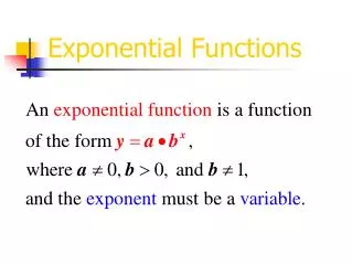
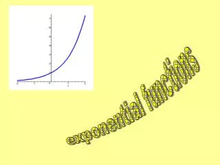
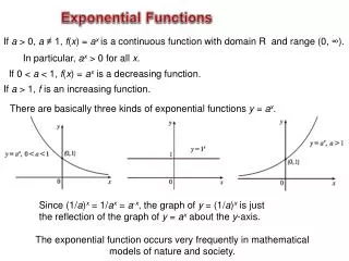
3. Exponential functions are of the form y = ax Why do all graphs of these functions pass through (0,1)? Go to graph ( or a graphical calculator) and plot y = 1x y = 2x y = 3x y = 4x What do you notice ? What happens between 2 and 3?

4. between 2 and 3 there is a number such that the gradient function would be the same as the function. this number is represented by the letter ‘e’. e ≈ 2.718 y = ex is often referred to as the exponential function if y then click here for more about e

5. population growth in real life is modelled by the graph of y = ex All exponential graphs follow a similar pattern. y = ex

6. if you were to draw up a table of values for this function you could see how rapidly it grows. also note: as x →∞ then ex→∞ when x = 0, e0 = 1 (0,1) lies on the curve as x →-∞ then ex→ 0 (it approaches but never reaches the x axis)

7. How about the graph of y = e-x this is a reflection of y = ex in the y-axis this graph is often referred to as exponential decay. it is used to model examples from real life such as the fall in value of a car as well as the decay in radioactive isotopes.

8. Sketching exponential graphs • calculate some values to get an idea of the shape • mark points where the axes are crossed for example y = 10e-x a table of values would give And the graph would look like this (0,10) y =10e-x 0

9. Solving Problems involving exponential decay and growth The price of a used car can be represented by the formula where P is the price in £’s and t is the age in years from new. Calculate: • the new price • the value at 5 years old What does the model suggest about the eventual value of the car? Use this to sketch the graph of P against t I will pause here while you work it out

10. you should have got: • when t = 0 then [remember e0 = 1] P = 16000 x 1 Price when new is £16000. b) when t = 5 P = £9704.49 Price after 5 years is £9704.49 c) as t →∞ → 0 therefore P → 0 the eventual value is £0 16000

11. Exercise 3A page 35

12. To go further we now need to look at the inverse of ex. The inverse function of ex is logex or lnx With this information we can plough on and solve equations.

13. Solve the equation ex = 7 Using the inverse operation gives x = ln7 Now solve lnx = 25 Taking the inverse gives x = e25

14. A bit harder now: Solve e2x+3 = 9 Taking inverses give 2x + 3 = ln9 2x = ln9 – 3 x = ½ln9 - x = ln3 - Remember ½ln9 = ln9½ =ln3

15. And now solve 2lnx + 1 = 5 Rearrange to get 2lnx = 4 lnx = 2 x = e2

16. We also need to be able to plot the graph of lnx and simple transformations of it

17. as x →0 then y →∞ • when x = 1, y = 0 (0,1) lies on the curve • lnx does not exist for negative numbers • as x →∞ then y → ∞ (slowly) The important facts about the graph y = lnx are:

18. Sketch the graph of y = ln(3 – x) Thinking this through: when x →3 , y → ∞ when x = 2 y = ln(3 – 2) = ln1 = 0 As x → -∞ , y → ∞ (slowly) So the graph will look like this

19. How about the graph of y = 3 + ln(2x) ? Thinking it through again: when x → 0 , y → ∞ when x = ½, y = 3 + ln1 = 3 As x → ∞ , y → ∞ (slowly) So the graph will look like this

20. Now try exercise 3B page 39