Download
1 / 20
200 likes | 269 Vues
Given the difficulty in carrying out flux measurements, the common practice is to parameterize the air-sea flux in terms of two more easily measured parameters: concentration gradient and wind speed. For instance, F x = ρ C x U (X a – X w /S) = ρ k (X a – X w /S)

E N D
Given the difficulty in carrying out flux measurements, the common practice is to parameterize the air-sea flux in terms of two more easily measured parameters: concentration gradient and wind speed. For instance, Fx = ρCx U (Xa – Xw/S) = ρ k (Xa – Xw/S) where (Xa - Xw /S) is the CO2 concentration gradient across the air-sea interface, S is the Henry’s law constant (solubility), Cx is the dimensionless bulk transfer coefficient and k = Cx U is the mass transfer or piston velocity. Much of the current and past efforts on air-sea gas transfer are directed at finding a globally valid representation of k. Historically, expressions of the form k(U) are common; recent efforts are looking at additional factors.
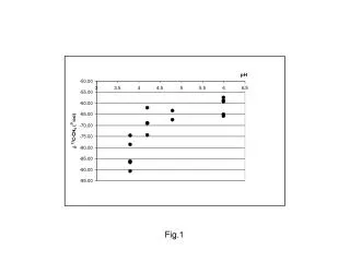
The first measurements of gas transfer rates were carried out by chemical engineers during the 1950s-60s. These laboratory experiments provided evidence that molecular diffusion in the diffusive sublayer below the surface was the rate limiting step. Early “stagnant” film models investigating the diffusive sublayer were based on k = Dx/h, where h is the thickness of the diffusive sublayer. h was found to decrease with increasing wind speed, or increasing subsurface turbulence. Note also the dependence of piston velocity on diffusivity. Note: the use of the “piston velocity” k instead of the dimensionless bulk coefficient Cx goes back to the Chemical Engineering roots of the problem. Broecker and Peng 1974, Fig 1
Subsequently, Jähne et al (1979, 1985), proposed k = function(u*, Dx, µ), where µ is the kinematic viscosity of water, and u* = is the friction velocity in water, Dimensional analysis yields: k/u* = f(µ/Dx) = f(Sc), where Sc = µ/Dx is the Schmidt number. Typically Sc = O(1000). Sc is a function of temperature and varies with gas. Based on laboratory experiments, Jähne et al (1979, 1985) proposed, k = f2(u* )Sc-n, with n = 2/3 for very light winds to n=1/2 for most conditions. Such a relationship allows data from different gases and temperatures to be compared. Data are normalised to a common Schmidt number, Sc =660 that of CO2 in 20oC sea water (or Sc=600, CO2 in 20oC fresh water): k660=kc (Sc660/Scc) -1/2
Methods for measuring CO2 flux: Chemical tracers Multiple tracer: Volatile (SF6, 3He) +conservative (BG:bacillus globigii var Niger), Nightingale et al., 2000: Global biogeochemical cycles ↓ k3He = ln (r1/r2) h /(t2-t1) where ri = 3He/BG at time ti h = depth Or, two volatile tracers: k3He-kSF6 = ln (r1/r2) h /(t2-t1) where ri = 3He/SF6 at time ti (k3He/kSF6 ) = (Sc3He/ScSF6 )n Sc = Schmidt Number, viscosity/gas diffusivity n ≈ -0.5
Methods for measuring CO2 flux (and k): Chemical tracers • (from Nightingale et al 2000) • it takes days - weeks for each flux estimate. While tracer methods provide useful estimates of gas-fluxes on scales of weeks, meteorological forcing conditions vary on scales of hours to days. Hence while tracer methods can not be used to improve our understanding of what factors control gas transfer.
Summary of tracer results, K660 vs U10 From Jähne and Haußecker 1998
Measuring CO2 flux • • Eddy correlation (or direct): • Requires fast measurement of the fluctuations of vertical velocity (w’) with those of CO2 (c’), humidity and temperature. • Need | pCO2a –pCO2w | > 40ppm for useful fluctuations on IRGA sensors • The Webb et al. 1980 correction is necessary because we measure not mixing ratio, but mass concentration which depends on density. The Webb correction requires the fluxes of sensible heat and humidity (or virtual temperature). • For water vapour, Webb correction is 0(3%); for CO2 it is 0(100%) Correction of Webb et al. (1980)
It is common to seek an expression in the form k660(U10N). This has the advantage that U measurements are readily available by satellite. Note large scatter from individual 30 min estimates Gas transfer velocities versus wind speed, for GASEX 2001 with other parameterizations (from McGillis et al 2004).
Does there exist a universal expression of the form k660(U10N) ? While there is general agreement between the various experiments at moderate wind speeds, this does not extend to high or low winds. First we look at understanding additional factors affecting gas transfer at low winds. Gas transfer velocities versus wind speed, for various experiments (from Frew et al 2004).
Plot of k660 versus wind speed for various surfactant levels. These are estimated from laboratory heat transfer experiments (Sc = 7). In the field, surfactants cease to be effective above 4 to 5 m/s. From Zappa et al , 2004 JGR
Plot of fractional coverage of microscale wave breaking, AB versus wind speed for different surfactants levels. These are estimated from laboratory heat transfer experiments (Sc = 7). From Zappa et al 2004
Plot of k660 versus fractional coverage of microscale wave breaking, AB. These are estimated from laboratory heat transfer experiments (Sc = 7) with different amounts of surfactant. From Zappa et al 2004 → At low winds gas transfer rates correlate well with microwave breaking
Plot of k660 versus mean square slope MSS of surface waves in various wavelength bands, <S2>. These are estimated from laboratory and field data with different amounts of surfactant. From Frew et al 2004, JGR → At low winds gas transfer rates correlate well with MSS of high frequency waves.
Area coverage microscale wave breaking is related to MSS, especially of the small waves. From Zappa et al 2004
The story at low winds: At low winds, the sea surface may be affected by affected by the presence of surfactants, either natural (organic) or manmade. These slicks dampen the small scale waves, and reduce microscale wave breaking. These in turn reduce surface renewal events, leading to a thicker diffusive sublayer and reduced gas transfer. Here, MSS is a better parameter than U for k. MSS can be also be measured by satellite (AB can not)
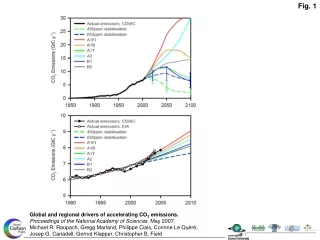
Breaking waves increase turbulence in the upper ocean, and provide a new mechanism for disrupting/thinning the diffusive sublayer. Lamont and Scott (1973) proposed a scaling for k in terms of the dissipation rate of turbulent kinetic energy, ε: k = const Sc-n (εμ)1/4 We can now measure k and ε, and will be testing this. Wave breaking in Hurricane Isabel, U ≈ 50m/s
Several different expression exist for bubble mediated transfer. From Woolf (1997), via Fairall et al 2002 (source of figure and text), Wave breaking in Hurricane Isabel, U ≈ 50m/s To date, none of the expressions have been well tested in the field. This is being done following two recent cruises: UK-SOLAS’ DOGEE 2007 and GASEX-3 in the Southern Ocean (2008) With bubbles w/o bubbles
+ Weekly multi-satellite wind field e.g. Bentamy et al 2003 + = Source: Takahashi et al.
For pCO2w, we rely on measurements. See the website http://cdiac.ornl.gov/oceans/LDEO_Underway_Database/LDEO_home.html
The source for these maps is pCO2w data collected from scientific ships And sometimes buoys. This map show all shiptracks over almost 40 years that go into the database. Not how few tracks there are in large areas of the ocean, particularly in the southern hemisphere. The LDEO pco2 maps account for this problem by averaging into 5 degx5deg boxes, interpolating in space, and interpolating in time (after accounting for seasonality and the interannual trend) Source: Takahashi et al.