Download
1 / 84
840 likes | 846 Vues
C. E. N. T. E. R. F. O. R. I. N. T. E. G. R. A. T. I. V. E. B. I. O. I. N. F. O. R. M. A. T. I. C. S. V. U. Master Course Sequence Alignment Lecture 13 Evolution/Phylogeny. Bioinformatics.

E N D
C E N T E R F O R I N T E G R A T I V E B I O I N F O R M A T I C S V U Master Course Sequence Alignment Lecture 13Evolution/Phylogeny
Bioinformatics • “Nothing in Biology makes sense except in the light of evolution” (Theodosius Dobzhansky (1900-1975)) • “Nothing in bioinformatics makes sense except in the light of Biology (and thus evolution)”
Content • Evolution • requirements • negative/positive selection on genes (e.g. Ka/Ks) • homology/paralogy/orthology (operational definition ‘bi-directional best hit’) • Clustering • single linkage • complete linkage • Phylogenetic trees • ultrametric distance (uniform molecular clock) • additive trees (4-point condition) • UPGMA algorithm • NJ algorithm • Character-based methods (Maximum Parsimony, ML) • bootstrapping
Darwinian Evolution What is needed: • Template (DNA) • Copying mechanism (meiosis/fertilisation) • Variation (e.g. resulting from copying errors, gene conversion, crossing over, genetic drift, etc.) • Selection
DNA evolution • Gene nucleotide substitutions can be synonymous (i.e. not changing the encoded amino acid) or nonsynonymous (i.e. changing the a.a.). • Rates of evolution vary tremendously among protein-codinggenes. Molecular evolutionary studies have revealed an∼1000-fold range of nonsynonymous substitution rates (Liand Graur 1991). • The strength of negative (purifying) selectionis thought to be the most important factor in determiningthe rate of evolution for the protein-coding regions of agene (Kimura 1983; Ohta 1992; Li 1997).
DNA evolution • “Essential” and “nonessential” are classic moleculargenetic designations relating to organismal fitness. • A gene is considered to be essential if a knock-outresults in (conditional) lethality or infertility. • Nonessential genes are those for which knock-outs yieldviable and fertile individuals. • Given the role of purifyingselection in determining evolutionary rates, thegreater levels of purifying selection on essential genes leads to a lower rate of evolution relative to that ofnonessential genes.
Ka/Ks Ratios • Ksis defined as the number of synonymous nucleotidesubstitutions per synonymous site • Ka is defined as the numberof nonsynonymous nucleotide substitutions per nonsynonymoussite • The Ka/Ks ratiois used to estimate the type of selection exerted on a given gene or DNA fragment • Need orthologousnucleotide sequence alignments • Observe nucleotide substitution patterns at given sites and correct numbers using, for example, the Pamilo-Bianchi-Limethod (Li 1993; Pamilo and Bianchi 1993). • Correction is needed because of the following: Consider the codons specifying aspartic acid and lysine: both start AA, lysine ends A or G, and aspartic acid ends T or C. So, if the rate at which C changes to T is higher from the rate that C changes to G or A (as is often the case), then more of the changes at the third position will be synonymous than might be expected. Many of the methods to calculate Ka and Ks differ in the way they make the correction needed to take account of this type of bias.
Ka/Ks ratios The frequency of different values of Ka/Ks for 835 mouse–rat orthologous genes. Figures on the x axis represent the middle figure of each bin; that is, the 0.05 bin collects data from 0 to 0.1
Ka/Ks ratios • Three types of selection: • Negative (purifying) selection Ka/Ks < 1 • Neutral selection (Kimura) Ka/Ks ~ 1 • Positive selection Ka/Ks > 1
Orthology/paralogy Orthologous genes are homologous (corresponding) genes in different species Paralogous genes are homologous genes within the same species (genome)
Orthology/paralogy • Operational definition of orthology: • Bi-directional best hit: • Blast gene A in genome 1 against genome 2: gene B is best hit • Blast gene B against genome 1: if gene A is best hit • A and B are orthologous • A number of other criteria is also in use (part of which is based on phylogeny)
Xenology • Xenologs result from the horizontal transfer of a gene between two organisms. • The function of xenologs can be variable, depending on how significant the change in context was for the horizontally moving gene. In general, though, the function tends to be similar (before and after horizontal transfer)
Multivariate statistics – Cluster analysis C1 C2 C3 C4 C5 C6 .. 1 2 3 4 5 Raw table Any set of numbers per column Similarity criterion Similarity matrix Scores 5×5 Cluster criterion Dendrogram
Multivariate statistics – Cluster analysisWhy do it? • Finding a true typology • Model fitting • Prediction based on groups • Hypothesis testing • Data exploration • Data reduction • Hypothesis generation But you can never prove a classification/typology!
Cluster analysis – data normalisation/weighting C1 C2 C3 C4 C5 C6 .. 1 2 3 4 5 Raw table Normalisation criterion C1 C2 C3 C4 C5 C6 .. 1 2 3 4 5 Normalised table Column normalisation x/max Column range normalise (x-min)/(max-min)
Cluster analysis – (dis)similarity matrix C1 C2 C3 C4 C5 C6 .. 1 2 3 4 5 Raw table Similarity criterion Similarity matrix Scores 5×5 Di,j= (k | xik – xjk|r)1/r Minkowski metrics r = 2 Euclidean distance r = 1 City block distance
Cluster analysis – Clustering criteria Similarity matrix Scores 5×5 Cluster criterion Dendrogram (tree) Single linkage - Nearest neighbour Complete linkage – Furthest neighbour Group averaging – UPGMA Ward Neighbour joining – global measure
Comparing sequences - Similarity Score - • Many properties can be used: • Nucleotide or amino acid composition • Isoelectric point • Molecular weight • Morphological characters • But: molecular evolution through sequence alignment
Multivariate statistics Producing a Phylogenetic tree from sequences 1 2 3 4 5 Multiple sequence alignment Similarity criterion Distance matrix Scores 5×5 Cluster criterion Phylogenetic tree
Evolution • Most of bioinformatics is comparative biology • Comparative biology is based upon evolutionary relationships between compared entities • Evolutionary relationships are normally depicted in a phylogenetic tree
Where can phylogeny be used • For example, finding out about orthology versus paralogy • Predicting secondary structure of RNA • Studying host-parasite relationships • Mapping cell-bound receptors onto their binding ligands • Multiple sequence alignment (e.g. Clustal)
Similarity criterion for phylogeny • ClustalW: uses sequence identity with Kimura (1983) correction: Corrected K = - ln(1.0-K-K2/5.0), where K is percentage divergence corresponding to two aligned sequences • There are various models to correct for the fact that the true rate of evolution cannot be observed through nucleotide (or amino acid) exchange patterns (e.g. back mutations) • Saturation level is ~94%, higher real mutations are no longer observable
Human -KITVVGVGAVGMACAISILMKDLADELALVDVIEDKLKGEMMDLQHGSLFLRTPKIVSGKDYNVTANSKLVIITAGARQ Chicken -KISVVGVGAVGMACAISILMKDLADELTLVDVVEDKLKGEMMDLQHGSLFLKTPKITSGKDYSVTAHSKLVIVTAGARQ Dogfish –KITVVGVGAVGMACAISILMKDLADEVALVDVMEDKLKGEMMDLQHGSLFLHTAKIVSGKDYSVSAGSKLVVITAGARQ Lamprey SKVTIVGVGQVGMAAAISVLLRDLADELALVDVVEDRLKGEMMDLLHGSLFLKTAKIVADKDYSVTAGSRLVVVTAGARQ Barley TKISVIGAGNVGMAIAQTILTQNLADEIALVDALPDKLRGEALDLQHAAAFLPRVRI-SGTDAAVTKNSDLVIVTAGARQ Maizey casei -KVILVGDGAVGSSYAYAMVLQGIAQEIGIVDIFKDKTKGDAIDLSNALPFTSPKKIYSA-EYSDAKDADLVVITAGAPQ Bacillus TKVSVIGAGNVGMAIAQTILTRDLADEIALVDAVPDKLRGEMLDLQHAAAFLPRTRLVSGTDMSVTRGSDLVIVTAGARQ Lacto__ste -RVVVIGAGFVGASYVFALMNQGIADEIVLIDANESKAIGDAMDFNHGKVFAPKPVDIWHGDYDDCRDADLVVICAGANQ Lacto_plant QKVVLVGDGAVGSSYAFAMAQQGIAEEFVIVDVVKDRTKGDALDLEDAQAFTAPKKIYSG-EYSDCKDADLVVITAGAPQ Therma_mari MKIGIVGLGRVGSSTAFALLMKGFAREMVLIDVDKKRAEGDALDLIHGTPFTRRANIYAG-DYADLKGSDVVIVAAGVPQ Bifido -KLAVIGAGAVGSTLAFAAAQRGIAREIVLEDIAKERVEAEVLDMQHGSSFYPTVSIDGSDDPEICRDADMVVITAGPRQ Thermus_aqua MKVGIVGSGFVGSATAYALVLQGVAREVVLVDLDRKLAQAHAEDILHATPFAHPVWVRSGW-YEDLEGARVVIVAAGVAQ Mycoplasma -KIALIGAGNVGNSFLYAAMNQGLASEYGIIDINPDFADGNAFDFEDASASLPFPISVSRYEYKDLKDADFIVITAGRPQ Lactate dehydrogenase multiple alignment Distance Matrix 1 2 3 4 5 6 7 8 9 10 11 12 13 1 Human 0.000 0.112 0.128 0.202 0.378 0.346 0.530 0.551 0.512 0.524 0.528 0.635 0.637 2 Chicken 0.112 0.000 0.155 0.214 0.382 0.348 0.538 0.569 0.516 0.524 0.524 0.631 0.651 3 Dogfish 0.128 0.155 0.000 0.196 0.389 0.337 0.522 0.567 0.516 0.512 0.524 0.600 0.655 4 Lamprey 0.202 0.214 0.196 0.000 0.426 0.356 0.553 0.589 0.544 0.503 0.544 0.616 0.669 5 Barley 0.378 0.382 0.389 0.426 0.000 0.171 0.536 0.565 0.526 0.547 0.516 0.629 0.575 6 Maizey 0.346 0.348 0.337 0.356 0.171 0.000 0.557 0.563 0.538 0.555 0.518 0.643 0.587 7 Lacto_casei 0.530 0.538 0.522 0.553 0.536 0.557 0.000 0.518 0.208 0.445 0.561 0.526 0.501 8 Bacillus_stea 0.551 0.569 0.567 0.589 0.565 0.563 0.518 0.000 0.477 0.536 0.536 0.598 0.495 9 Lacto_plant 0.512 0.516 0.516 0.544 0.526 0.538 0.208 0.477 0.000 0.433 0.489 0.563 0.485 10 Therma_mari 0.524 0.524 0.512 0.503 0.547 0.555 0.445 0.536 0.433 0.000 0.532 0.405 0.598 11 Bifido 0.528 0.524 0.524 0.544 0.516 0.518 0.561 0.536 0.489 0.532 0.000 0.604 0.614 12 Thermus_aqua 0.635 0.631 0.600 0.616 0.629 0.643 0.526 0.598 0.563 0.405 0.604 0.000 0.641 13 Mycoplasma 0.637 0.651 0.655 0.669 0.575 0.587 0.501 0.495 0.485 0.598 0.614 0.641 0.000 How can you see that this is a distance matrix?
Cluster analysis – Clustering criteria Similarity matrix Scores 5×5 Cluster criterion Dendrogram (tree) Four different clustering criteria: Single linkage - Nearest neighbour Complete linkage – Furthest neighbour Group averaging – UPGMA Neighbour joining (global measure) Note: these are all agglomerative cluster techniques; i.e. they proceed by merging clusters as opposed to techniques that are divisive and proceed by cutting clusters
General agglomerative cluster protocol • Start with N clusters of 1 object each • Apply clustering distance criterion and merge clusters iteratively until you have 1 cluster of N objects • Most interesting clustering somewhere in between distance Dendrogram (tree) Note: a dendrogram can be rotated along branch points (like mobile in baby room) -- distances between objects are defined along branches 1 cluster N clusters
Single linkage clustering (nearest neighbour) Char 2 Char 1
Single linkage clustering (nearest neighbour) Char 2 Char 1
Single linkage clustering (nearest neighbour) Char 2 Char 1
Single linkage clustering (nearest neighbour) Char 2 Char 1
Single linkage clustering (nearest neighbour) Char 2 Char 1
Single linkage clustering (nearest neighbour) Char 2 Char 1 Distance from point to cluster is defined as the smallest distance between that point and any point in the cluster
Single linkage clustering (nearest neighbour) Char 2 Char 1 Distance from point to cluster is defined as the smallest distance between that point and any point in the cluster
Single linkage clustering (nearest neighbour) Let Ci andCj be two disjoint clusters: di,j = Min(dp,q), where p Ci and q Cj Single linkage dendrograms typically show chaining behaviour (i.e., all the time a single object is added to existing cluster)
Complete linkage clustering (furthest neighbour) Char 2 Char 1
Complete linkage clustering (furthest neighbour) Char 2 Char 1
Complete linkage clustering (furthest neighbour) Char 2 Char 1
Complete linkage clustering (furthest neighbour) Char 2 Char 1
Complete linkage clustering (furthest neighbour) Char 2 Char 1
Complete linkage clustering (furthest neighbour) Char 2 Char 1
Complete linkage clustering (furthest neighbour) Char 2 Char 1
Complete linkage clustering (furthest neighbour) Char 2 Char 1 Distance from point to cluster is defined as the largest distance between that point and any point in the cluster
Complete linkage clustering (furthest neighbour) Char 2 Char 1 Distance from point to cluster is defined as the largest distance between that point and any point in the cluster
Complete linkage clustering (furthest neighbour) Let Ci andCj be two disjoint clusters: di,j = Max(dp,q), where p Ci and q Cj More ‘structured’ clusters than with single linkage clustering
Clustering algorithm • Initialise (dis)similarity matrix • Take two points with smallest distance as first cluster • Merge corresponding rows/columns in (dis)similarity matrix • Repeat steps 2. and 3. using appropriate cluster measure until last two clusters are merged
Phylogenetic trees MSA quality is crucial for obtaining correct phylogenetic tree 1 2 3 4 5 Multiple sequence alignment (MSA) Similarity criterion Similarity/Distance matrix Scores 5×5 Cluster criterion Phylogenetic tree
Phylogenetic tree (unrooted) human Drosophila internal node fugu mouse leaf OTU – Observed taxonomic unit edge
Phylogenetic tree (unrooted) root human Drosophila internal node fugu mouse leaf OTU – Observed taxonomic unit edge
Phylogenetic tree (rooted) root time edge internal node (ancestor) leaf OTU – Observed taxonomic unit Drosophila human fugu mouse Clade - group of two or more taxa that includes both their common ancestor and all of their descendents.
How to root a tree m f • Outgroup – place root between distant sequence and rest group • Midpoint – place root at midpoint of longest path (sum of branches between any two OTUs) • Gene duplication – place root between paralogous gene copies (see earlier globin example) h D f m h D 1 m f 3 1 2 4 2 3 1 1 1 h 5 D f m h D f- f- h- f- h- f- h- h-