Download
1 / 18
190 likes | 300 Vues
Estimating aboveground biomass: remote sensing approach Daolan Zheng Dept. of EEES, University of Toledo. Abstract *** Aboveground biomass (AGB)—2.5 cm dbh for stands > 5 yrs and > 1.3 m for stands < 5 yrs.

E N D
Estimating aboveground biomass: remote sensing approach Daolan Zheng Dept. of EEES, University of Toledo
Abstract *** Aboveground biomass (AGB)—2.5 cm dbh for stands > 5 yrs and > 1.3 m for stands < 5 yrs. *** Bridges applications of remote sensing (RS) with forest practices in Chequamegon National Forest, WI by producing high-resolution maps of age and AGB. *** We coupled AGB values, calculated from tree dbh., with RS indices to produce initial biomass map (IBM). *** The IBM was overlaid with cover map to generate age map using biomass threshold values for each age category (e.g. young, intermediate and mature) based on field data and frequency analysis of IBM. *** Hardwood forests--stand age and NIR (r2 = 0.95). *** Pine forests were strongly related to NDVIc (r2 = 0.86) *** The total AGB in 2001 = 3.3 million metric tons (dry weight), 76.5% of which was in hardwood and mixed hardwood/pine forests. Ranged from 1 to 358 Mg/ha with an average of 70 and standard deviation of 54 Mg/ha. The modal AGB class 81-100 Mg/ha (16.1%). 200 Mg/ha < 3% (mature HW). *** Validation (R2 = 0.67, p < 0.001). The AGB and age maps can be used for quantifying the regional carbon budget, fuel accumulation, or monitoring management practices.
Introduction AGB is a necessary component for studying productivity, carbon cycles, nutrient allocation, and fuel accumulation; RS techniques allow to examine properties and processes of ecosystems and their inter-annual variability at multiple scales because of ability to observe large areas/high re-visitation frequencies; Success in estimating forest biomass/production using RS reported worldwide. The models need local calibration with ground data; Spectral Vegetation Index (SVI), Simple Ratio (SR), NDVI, and NDVIc are useful Xs for estimating LAI/biomass/productivity; Stand-level AGB is a function of species composition, tree height, basal area, and stand structure, but dbh. is the most commonly used variable. Species-based biomass models are accurate at tree/plot/stand but can’t be used across the landscape for pattern analysis unless linked to RS data. Combining carbon pool assessments from existing inventories with RS variables is one of priorities identified in the NACP. Research gaps--lack of a high-resolution stand-age map for ecological analyses in the CNF. The existing USDA stand-age map developed for other purposes has coarse spatial resolution, limited availability, and is infrequently updated.
Overall objectives: Combining field observations and RS data to 1) produce a high-resolution age map; 2) generate a spatially explicit AGB map; and 3) examine spatial patterns of AGB in CNF. • Three specific steps: • estimation of initial AGB by coupling field measurements with solely RS data through stepwise regressions for HW, pine forests, and both; • obtaining a landscape age map by overlaying the initial AGB map with an existing land-cover map using biomass threshold values, determined by frequency analysis and field observations, to separate Y/INTER/MATURE hardwood and pine forests; • refining the initial landscape AGB estimates using a combination of newly developed models incorporating age variable.
Methods • Study area CNF, WI ; • Climate—Annual mean of 4.7 (0C) with a short/hot summer and cold winter, Growing season (120-140 days), PPT 660-700mm/yr; • Soil--Wisconsin-age glaciated landscape with deep, coarse-textur; • Topography--flat to rolling (Ele. 232-459 m); • Cover types—HW, JP, RP, MIX, RFS, and NFBG (Bresee et al. (2004). Forests were harvested at an average age between 65 – 70 years (USDA, 1986), resulted in more or less the even age forest structure. • 2) Field design and measurements of tree dbh • a) Model development: 55 circular plots (2002). Continuous stands--2.6 km2 for M/INTER and 1.3 km2 for Y and CC across cover types (i.e., RP, JP and HW). In each type, 4 age classes were sampled (i.e., 3-8, 15-20, 32-40, and 65-75 years), total of 12 stands. In each stand, 4-5 plots were set around its center. All plots (except for young hardwood, 0.01 ha) was approximately 0.05-ha. Within each 0.05-ha plot the dbh. of all trees (> 2.5 cm dbh.) and the average stand age of the plot was determined by tree-ring analysis and recorded. 1.3 m taller for YHW.
Continued with METHODS • Validation: 40 additional plots were selected in 2003 following the same criteria as in 2002. Once a suitable stand was found, a random number table was used to determine plot location (i.e., compass bearing and distance). dbh. of the trees in each sub area (i.e., 0.05 or 0.01 ha) were measured and adjusted • 3) Biomass estimation • Models (species-based) developed in the area used first, if not available the ones from the geographically closest regions were used. • 4) Remotely sensed indices • The image was geo-rectified to UTM and the raw satellite data in each ETM+ band (except thermal and panchromatic) were converted to reflectance using an exo-atmospheric model. • Six individual bands (B, G, R, NIR, and 2 middle infrared), and 5 vegetation indices including: 1) ratio of blue/red, 2) NDVI (NIR – red) / (NIR + red), (Rouse et al., 1973), 3) simple ratio (NIR/red), 4) Modified Soil Adjusted Vegetation Index (MSAVI) = (ρNIR – ρred) / (ρNIR – ρred + L) * (1 + L), L is a soil-adjustment factor (Qi et al., 1994), and 5) NDVIc calculated from NDVI * [1 – (mIR – mIRmin) / (mIRmax – mIRmin)] (Nemani et al., 1993).
Continued with METHODS 5) Relating ground data with RS products to produce maps of initial AGB, age, and final AGB
RESULTS Remote-sensing derived variables including MSAVI, bands of red, near-infrared (NIR), and middle-infrared (MIR), were useful predictors of AGB (Table 2). The overall model explained 82% of variance (a=0.001). However, better models were achieved by separating the plots into hardwood and pine forests. Hardwood AGB was strongly related to stand age and NIR (r2 = 0.95) using a linear model, while AGB for pine forests was strongly related to NDVIc using a sigmoidal model (r2 = 0.86). Statistic models used for calculating aboveground biomass (AGB, Mg/ha). __________________________________________________________________ Models Description N r2 AGB = 48.8 * (NIR/red) + 2.3 * Age – 454 * MASVI - 38 Overall 55 0.82 AGB = 111 * (NDVIc10.3 / (NDVIc10.3 + 0.3510.3)) Pine 35 0.86 AGB = 232.5 * NIR + 2.7 * Age – 71 Hardwood 20 0.95
The final predicted AGB values across the landscape ranged from 1 to 358 Mg/ha (mean = 70 Mg/ha and Std.== 54 Mg/ha, total = 3.3 million tons dry weight). Spatially, low AGB occurred in RFS and CC areas while high AGB occurred in mature hardwood forests.
The AGB class with the highest frequency (16.1%) was 80-100 Mg/ha. The distribution was skewed toward lower values due to landscape structure. < 3% of the landscape had AGB > 200 Mg/ha.
*** Hardwood and mixed forests contained approximately 77% of the total AGB while PB stored less than 3%; *** Pine forests comprised about 20% of the total AGB across the landscape. *** Mean AGB value of red pine (57 Mg/ha) was about 33% higher than that of jack pine (43 Mg/ha). Clearcuts had the lowest values in terms of both mean AGB and proportion of total AGB (0.3%). Among the cover types, the AGB estimates for hardwood had the largest variation (Std = 60 Mg/ha) while the estimates for jack pine had the smallest variation (Std = 33 Mg/ha).
The final estimated AGB values compared reasonably with the independent field observations in the forty validation plots (R2=0.67, p = 0.001).
Discussion NDVIc proved to be a good predictor for pine forest. The majority of pine forests in the study area were classified as young and intermediate ages with open canopy structures at some degrees. Stand age is a strong predictor in estimating AGB of HW forests in the area. (R2 = 0.67 vs. R2 = 0.56). Two separate lines are needed for veg. Index if one or more infrared bands involved in the GLR. Separating improved the AGB predictions (50% more in NIR for HW due to different canopy structures). The classification system for age map was defined to be meaningful for fuel loading. CC were divided into pine-forest clearcuts (CCP) and CCH. Hardwood forests usually retained more available fuel on the floor, pine much less. Our models tended to underestimate the AGB at high and overestimate at low end. The estimated AGB values corresponded well in general with previously studies lower/upper (60-600 Mg/ha AGB for mature forests, Crow, 1978). 3 HW sites ranged from 94 to 119 Mg/ha (ours 93 ± 60 Mg/ha). Our AGB estimates corresponded well with Brown et al. (1999), but caution must be taken because: 1) Total vs AGB, 2) county (broader classes) vs. 30 m so can’t be compared. It is likely that high spatial resolution inputs are more suitable for landscape level analysis. Potential errors could be from land-cover map, sampling errors, confounding effects of soil moisture and soil color, and model utilization, 6:4 ratio for mixed forests. Biomass models--errors 3.2% for Red oak, 20% for Sugar maple, mean=12.5%. AGB estimates may be improved by incorporating tree height using Lidar.
Conclusions The AGB map may be used to refine the land cover classification by differentiating young hardwood forests from the mature ones. Our AGB map can be a useful source for estimating aboveground net primary production (ANPP). A good relationship exists between AGB estimates and ANPP before forest stands reach old stage (Euskirchen et al., 2002). Fuel accumulation in forest ecosystems can be theoretically determined by ANPP and the decomposition rate (Ryu et al., 2003). This study provides needed baseline information for landscape level analyses relating to regional carbon budget (i.e., monitoring changes of carbon pool over time).
Acknowledgements This research is supported by the USDA Joint Fire Science Project. I thank the following individuals for field data collection and preparation of the manuscript: John Rademacher, Jiquan Chen, Thomas Crow, Mary Bresee, James Le Moine, and Soung-Ryoul Ryu