Download
1 / 60
620 likes | 998 Vues
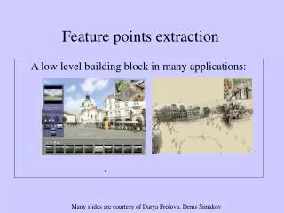
Feature points extraction. A low level building block in many applications: Structure from motion Object identification: Video Google Objects recognition . . Many slides are courtesy of Darya Frolova, Denis Simakov. A motivating application Building a panorama.

E N D
Feature points extraction A low level building block in many applications: Structure from motion Object identification: Video Google Objects recognition. Many slides are courtesy of Darya Frolova, Denis Simakov
A motivating application Building a panorama • We need to match/align/register images
Building a panorama 1) Detect feature points in both images
Building a panorama • Detect feature points in both images • Find corresponding pairs
Building a panorama • Detect feature points in both images • Find corresponding pairs • Find a parametric transformation (e.g. homography) • Warp (right image to left image)
2 (n) views geometry Today's talk Matching with Features • Detect feature points in both images • Find corresponding pairs • Find a parametric transformation
Criteria for good Features Repeatable detector Distinctive descriptor Accurate 2D position
Repeatable detector • Property 1: • Detect the same point independently in both images no chance to match!
Distinctive descriptor • Property 2: • Reliable matching of a corresponding point ?
Accurate 2D position • Property 3: Localization • Where exactly is the point ? Sub-pixel accurate 2D position
Examples of commonly used features • Harris, Corner Detector (1988) • KLT Kanade-Lucas-Tomasi (80’s 90’s) • Lowe, SIFT (Scale Invariant Features Transform) • Mikolajczyk &Schmid, “Harris Laplacian” (2000) • Tuytelaars &V.Gool. Affinely Invariant Regions • Matas et.al. “Distinguished Regions” • Bay et.al. “SURF” (Speeded Up Robust Features) (2006)
Detection: points with high “Cornerness” (next slide) Descriptor: a small window around it (i.e., matching by SSD, SAD) Corner detectors Harris & KLT Localization: peak of a fitted parabola that approximates the “cornerness” surface C.Harris, M.Stephens. “A Combined Corner and Edge Detector”. 1988 Lucas Kanade. An Iterative Image Registration Technique 1981. Tomasi Kanade. Detection and Tracking of Point Features.1991. Shi Tomasi. Good Features to Track 1994.
“Cornerness” R (x0, y0) of a point is defined as: Cornerness(formally) where M is a 22 “structure matrix” computed from image derivatives: And k – is a scale constant, and w(x,y) is a weight function
Descriptors & Matching • Descriptors ROI around the point (rectangle / Gaussian ) typical sizes 8X8 up to 16X16. • Matching: (representative options) • Sum Absolute Difference • Sum Square Difference • Correlation (Normalized Correlation)
Localization • Fit a surface / parabola P(x,y) (using 3x3 R values) • Compute its maxima • Yields a non integer position.
Harris corner detector is motivated by accurate localization Find points such that: small shift high intensity change Hidden assumption: Good localization in one image good localization in another image
Window function Shifted intensity Intensity E Window function w(x,y) = or 1 in window, 0 outside Gaussian u v Cornerness ≈ High change of intensity for every shift Harris Detector Cont. Change of intensity for the shift [u,v]:
Harris Detector: Basic Idea “flat” region: “edge”: “corner”:
Measuring the “properties” of E() M depends on image properties
“properties” of E() ↔ “properties” of M Harris Detector Cont. For small shifts [u,v] we have a bilinear approximation: where M is a 22 matrix computed from image derivatives:
Bilinear form and its eigenvalue 1, 2 – eigenvalues of M Ellipse E(u,v) = const direction of the slowest change direction of the fastest change (min)-1/2 (max)-1/2
“Cornerness” of a point R(x0, y0) is defined as: KLT And k – is a scale constant, and w(x,y) is a weight function
Classification of image points using eigenvalues of M: 2 “Edge” 2 >> 1 “Corner”1 and 2 are large,1 ~ 2;E increases in all directions 1 and 2 are small;E is almost constant in all directions “Edge” 1 >> 2 “Flat” region 1
“Cornerness” of a point R(x0, y0) > threshold >0: And 0<k<0.25 (~0.05) is a scale constant, Harris corner detector Computed using 2 tricks: C.Harris, M.Stephens. “A Combined Corner and Edge Detector”. 1988
Harris Detector 2 “Edge” “Corner” • R depends only on eigenvalues of M • R is large for a corner • R is negative with large magnitude for an edge • |R| is small for a flat region R < 0 R > 0 “Flat” “Edge” |R| small R < 0 1
Harris Detector (summary) • The Algorithm: • Detection: Find points with large corner response function R (R > threshold) • Localization: Approximate (parabola) local maxima of R • Descriptors ROI around (rectangle) the point. Matching : SSD, SAD, NC.
Harris Detector: Workflow Compute corner response R
Harris Detector: Workflow Find points with large corner response: R>threshold
Harris Detector: Workflow Take only the points of local maxima of R
If I detected this point Will I detect this point If I detected this point Will I detect this point If I detected this point Will I detect this point Detector Properties Properties to be “Invariant” to 2D rotations Illumination Scale Surface orientation Viewpoint (base line between 2 cameras)
Harris Detector: Properties • Rotation invariance Ellipse rotates but its shape (i.e. eigenvalues) remains the same Corner response R is invariant to image rotation
R R threshold x(image coordinate) x(image coordinate) Harris Detector: Properties • Partial invariance to intensity change • Only derivatives are used to build M => invariance to intensity shift I I+b
Harris Detector: Properties • Non-invariant to image scale! points “classified” as edges Corner !
Harris Detector: Properties • Non-invariant for scale changes Repeatability rate is: # correspondences# possible correspondences “Correspondences” in controlled setting (i.e., take an image and scale it) is trivial C.Schmid et.al. “Evaluation of Interest Point Detectors”. IJCV 2000
Rotation Invariant Detection • Harris Corner Detector C.Schmid et.al. “Evaluation of Interest Point Detectors”. IJCV 2000
Examples of commonly used features • Harris, Corner Detector (1988) • KTL Kanade-Lucas-Tomasi • Lowe, SIFT (Scale Invariant Features Transform) • Mikolajczyk &Schmid, “Harris Laplacian” (2000) • Tuytelaars &V.Gool. Affinely Invariant Regions • Matas et.al. “Distinguished Regions” • Bay et.al. “SURF” (Speeded Up Robust Features) (2006)
Scale Invariant problem illustration • Consider regions (e.g. circles) of different sizes around a point
Scale invariance approach • Find a “native” scale. The same native scale should redetected (at images of different scale).
scale Laplacian y x Harris Scale Invariant Detectors • Harris-LaplacianFind local maximum of: Harris corner detector for set of Laplacian images 1 K.Mikolajczyk, C.Schmid. “Indexing Based on Scale Invariant Interest Points”. ICCV 2001
SIFT (Lowe) • Find local maximum of Difference of Gaussians scale DoG y x DoG D.Lowe. “Distinctive Image Features from Scale-Invariant Keypoints”. IJCV 2004
Difference of Gaussians images Kernels: • Functions for determining scale (Difference of Gaussians) where Gaussian Note: both kernels are invariant to scale and rotation
SIFT Localization • Fit a 3D quadric D(x,y,s) (using 3x3X3 DoG values) • Compute its maxima • Yields a non integer position (in x,y) . Brown and Lowe, 2002
D(x,y,s) is also used for pruning non-stable maxima D.Lowe. “Distinctive Image Features from Scale-Invariant Keypoints”. IJCV 2004
Scale Invariant Detectors • Experimental evaluation of detectors w.r.t. scale change Repeatability rate: # correspondences# possible correspondences K.Mikolajczyk, C.Schmid. “Indexing Based on Scale Invariant Interest Points”. ICCV 2001
SIFT – Descriptor • A vector of 128 values each between [0 -1] We also computed location scale “native” orientation D.Lowe. “Distinctive Image Features from Scale-Invariant Keypoints”. IJCV 2004
“native” orientation • Peaks in a gradient orientation histogram Gradient is computed at the selected scale 36 bins (resolution of 10 degrees). Many times (15%) more than 1 peak !? The “weak chain” in SIFT descriptor. D.Lowe. “Distinctive Image Features from Scale-Invariant Keypoints”. IJCV 2004
Computing a SIFT descriptor • Determine scale (by maximizing DoG in scale and in space), • Determine local orientation (direction dominant gradient). define a native coordinate system. • Compute gradient orientation histograms (of a 16x16 window) • 16 windows 128 values for each point/ (4x4 histograms of 8 bins) • Normalize the descriptor to make it invariant to intensity change D.Lowe. “Distinctive Image Features from Scale-Invariant Keypoints”. IJCV 2004