Download
1 / 42
420 likes | 546 Vues
Decision Theory. Varsha Varde. Introduction. Decision theory provides a rational methodology for making management decisions. It does not generate alternative courses of action It merely provides a rational way of choosing among several alternative strategies. Examples.

E N D
Decision Theory Varsha Varde
Introduction • Decision theory provides a rational methodology for making management decisions. • It does not generate alternative courses of action • It merely provides a rational way of choosing among several alternative strategies.
Examples • Natural Resource Development -Should an oil or gas well be drilled -What set of seismic experiment be run -What is the expected payoff of the investment in exploration • Agricultural applications -What crops should be planted -Should excess acreage be planted -What actions should be taken to fight pests
Examples • Financial Applications -What is the proper investment portfolio -What capital investments should be made this year -Whether to grant or not to grant credit to a customer • Marketing Applications -Which new product should be introduced -What is the best distribution channel to use -What is the best inventory strategy
Examples • Production Applications -Which of several different types of machines should be purchased -What maintenance schedule should be used -What mix of products should be produced
Assumptions • The decision maker can define all decision alternatives or strategies or acts which are being considered. The decision maker has a control over choice of these • He can define various states of nature or events for the decision setting which are not under his control -various economic conditions -various decisions of competitors -various weather conditions • He can estimate quantitatively benefits or costs of any decision alternative with various states of nature. These are called payoffs. • The problem is to choose the best of the alternatives to optimise the pay-offs
Conditions Under which Decisions are made • Decision making under conditions of certainty- Decision maker is certain as to which state of nature is going to occur • Decision making under conditions of uncertainty-No knowledge of the likelihood of the occurrence of various states of nature • Decision making under conditions of risks-has sufficient knowledge of the states of nature to assign probabilities to their occurrence
Conditions of Certainty • Conditions of certainty are rare. • Decision is easy under conditions of certainty
Illustration • A mineral water company has to make selection from amongst three strategies A , B and C • The three states of nature for decision setting are S1 ,S2 and S3 • Benefits of each option are known
Illustration Company has three strategy options: • A: Revolutionize product & high price (Oxygen enriched, vitamin fortified mineral water) • B: Modify packaging & small price increase (300 ml easy-to-slip-into-purse-or-pocket bottle) • C: Change design & marginal price hike (Four colour attractive picture on the lable).
Illustration Three possible states of nature are • S1: Huge increase in sales • S2: No change in sales • S3: Decline in sales
Certainty • Under conditions of certainty we have to choose an alternative which gives us maximum profit • Solution • Under S1 select option A (Rs 7,00,000) • Under S2 select option B (Rs 4,50,000) • Under S3 select option C (Rs 3,00,000)
Uncertainty • States of nature known but probability of their occurrence not known • Selection depends on whether decision maker is pessimistic or optimistic
MAXIMIN and MAXIMAX CRITERION • Pessimistic decision maker first identifies lowest profit with each decision alternative and chooses that alternative which gives maximum of the minimum profits. This criterion is called MAXMIN criterion • Optimistic decision maker first identifies highest profit with each decision alternative and chooses that alternative which gives maximum of the maximum profits. This criterion is called MAXIMAX criterion
Illustration of Maximin • Minimum Benefit from A : Rs. 1,50,000 • Minimum Benefit from B : Rs. 0 • Minimum Benefit from C : Rs. 3,00,000 • The Maximum of the three minimum benefits is Rs. 3,00,000 for C • Hence, Maximin criterion directs you to select option # C: Change design & marginal price hike.
Illustration of Maximax • Maxmum Benefit from A : Rs. 7,00,000 • Maxmum Benefit from B : Rs. 5,00,000 • Maxmum Benefit from C : Rs. 3,00,000 • The Maximum of the three maximum benefits is Rs. 7,00,000 for A • Hence, Maximax criterion directs you to select option # A: Revolutionize product & high price.
Hurwicz Criterion • Inventor: L. Hurwitz • Decision maker is neither optimistic nor pessimistic • He specifies Index of optimism which lies between0 and 1. • Weighted profits are calculated as (maximum profit for alternative)+ (1- )(minimum profit for alternative • Alternative which gives maximum of weighted profits is the decision chosen
Hurwitz Criterion • Let = 0.6 • Weighted profits are calculated as 0.6(maximum profit for alternative)+ 0.4(minimum profit for alternative) • Alternative which gives maximum of weighted profits is the decision chosen
Illustration of Hurwitz • Weighted Benefit from A : 0.6( 7,00,000)+.4(1,50,000)= 4,80,000 • Weighted Benefit from B : 0.6( 5,00,000)+.4(0)= 3,00,000 • Weighted Benefit from C : 0.6( 3,00,000)+.4(3,00,000)= 3,00,000 • The Maximum of the three weighted benefits is Rs. 4,80,000 for A • Hence, Hurwitz criterion directs you to select option # A: Revolutionize product & high price.
Minimax Regret Criterion • Inventor: L. J. Savage • Assumption: You may regret your decision afterwards (after-thought) • Hence, it is designed to select the option that MINIMIZES the MAXIMUM regrets • Determine ‘maximum regrets’ that can accrue from implementation of each option • Select the one for which it is lowest.
Minimax Regret Criterion • Regret is the opportunity loss or opportunity cost • Loss incurred by not selecting the best alternative • It is measured by the difference between the maximum profit we would have realised in case of known state of nature and the profit we realize
Illustration of Minimax Criterion • Maximum Regret from A : Rs. 1,50,000 • Maximum Regret from B : Rs. 3,00,000 • Maximum Regret from C : Rs. 4,00,000 • The Minimum of the three maximum regrets is Rs. 1,50,000 for A • Hence, Savage’s Minimax Regret criterion directs you to select option # A: Revolutionize product & fix high price.
Laplace Criterion • First three criteria are based on the best or worst outcome. They ignore the others. • Laplace Principle: ‘Don’t ignore any info.’ • Assign equal probability to all possible outcomes of each strategic option • Compute Expected Value of each option • Select the one for which EV is highest.
Decision Making Under Risk • All possible states of nature are known • Probabilities can be assigned to their likelihood of occurrence • Probabilities could be subjective based upon decision maker’s feelings and experience or • Probabilities could be objective based upon collection and analysis of numerous data related to states of nature • Expected values are used to evaluate decisions under uncertainty • Alternative with Maximum EMV is selected
Illustration Under Risk • Let P(S1)=0.5, P(S2)=0.3 and P(S3)=0.2 • EMV(A)=.5x700+.3x300+.2X150= 470 • EMV(B)=.5x500+.3x450+.2x0=400 • EMV(C)=.5x300+.3x300+.2x300=300 • Alternative A is selected
Expected Value Of Perfect Information • Accurate and complete information about future is known as perfect information. • When perfect information is available (at additional cost) the decision maker would select that alternative which has maximum profit under the known state of nature .This is known as conditional profit • The maximum possible expected profit is worked out as weighted average of conditional profits with weights as probabilities of various states of nature. This is called Expected profit under certainty • The expected value of perfect information is the difference between the expected profit under certainty and the best expected profit without perfect information
Conditional Profit Table Under Certainty & EPVI • Let P(S1)=0.5, P(S2)=0.3 and P(S3)=0.2 UNDER PERFECT INFORMATION • P(S1)EMV(Decision/S1)=.5x700= 350 • P(S2)EMV(Decision/S2)=.3x450 =135 • P(S3)EMV(Decision/S3)=.2x300 = 60 • EMV under certainty =545 • EMV under risk=470 • EVPI=545-470=75
Decision Tree Analysis • Decision tree is a mathematical model of decision situations • It guides a manager to arrive at a decision in an orderly fashion • It contains decision nodes from which one of several alternatives may be chosen • It contains state of nature nodes out of which one state of nature would occur • The tree is constructed starting from left & moving towards right • Problem represented by a decision tree is solved from right to left
Decision Tree • Identify all decision alternatives & their order • Identify chance events or states of nature that can occur after each decision • Develop a tree diagram showing the sequence of decisions & states of nature. • Obtain probability estimates of each state of nature • Obtain esimates of the consequences of all possible decisions & states of nature • Calculate expected value of all possible decisions • Select decision offering most attractive expected value
Illustration • A company has to take a decision to either expand by opening a new outlet or to maintain the current status. In case the company decides to expand it will earn an additional profit of Rs 30 lakh provided the economy grows. However if the economy declines the company will lose Rs 50 lakh. In case company maintains status-quo it will neither gain or lose. Draw a decision tree &state the best action under the assumption of 70% chance of economic growth. Also work out the action under 50% chance of economic growth.
Process Expected outcomeRs 30,00,000 Economic growth rises 0.7 Expand by opening new outlet Expected outcome – Rs 50,00,000 Economic growth declines 0.3 Maintain current status Rs 0 The circle denotes the point where different outcomes could occur. The estimates of the probability and the knowledge of the expected outcome allow the firm to make a calculation of the likely return. In this example it is: Economic growth rises: 0.7 x Rs 30,00,000 = Rs 21,00,000 Economic growth declines: 0.3 x – Rs 50,00,000 = – Rs 15,00,000 Calculation suggests it is wise to go ahead with the decision: net ‘benefit’ of +Rs 6,00,000 A square denotes the point where a decision is made, Here, they are contemplating opening a new outlet. The uncertainty is the state of the economy. If the economy continues to grow healthily the option is estimated to yield profits of Rs 30,00,000. However, if it fails to grow as expected, the potential loss is estimated at Rs 50,00,000. There is also the option to do nothing and maintain the current status quo! This would have an outcome of Rs 0.
Process Expected outcomeRs 30,00,000 Economic growth rises 0.5 Expand by opening new outlet Expected outcome – Rs 50,00,000 Economic growth declines 0.5 Maintain current status Rs 0 Look what happens however if the probabilities change. If the firm is unsure of the potential for growth, it might estimate it at 50:50. In this case the outcomes will be: Economic growth rises: 0.5 x Rs 30,00,000 = Rs 15,00,000 Economic growth declines: 0.5 x – Rs 50,00,000 = – Rs 25,00,000 In this instance, the net benefit is –Rs 10,00,000. The decision looks less favourable!
Marginal Analysis At a particular activity level • Marginal Profit (MP): Additional profit generated by increasing activity level by one unit • Marginal loss (ML) :Loss incurred by increasing activity level by one unit and not profiting by it • Probability (P) of generating additional profit by increasing activity level by one unit • Probability(1-P) of incurring loss by increasing activity level by one unit • Expected (MP)= P x MP • Expected (ML)=(1-P) x ML • Optimum level of activity occurs when Expected (MP)=Expected (ML) P x MP=(1-P)xML thus optimum level of activity P* is P*=ML/(ML+MP) • P* represents the minimum required probability to justify increase in activity level by one unit
Marginal Analysis • Let initial stock be x units. Increase it to (x+1) units • There would either be profit MP with probability P or loss ML with probability 1-P • Then P=P(D>X) and 1-P=P(D≤ X) • Optimum level of stock occurs when Expected (MP)=Expected (ML) P x MP=(1-P)xML P*=ML/(ML+MP) • P(D>X)= ML/(ML+MP)
Illustration • Classic Burger Shoppe sells chicken burgers. The cost of preparation comes to Rs11 and selling price is Rs 18.Demand for burger is normally distributed with mean 190 and SD 40.How many burgers should shop prepare so as to reduce losses from spoilage ? • We work out minimum required probability P* to justify preparation of an additional burger
MP=7 ,ML=11 P*=11/11+7=11/18= 0.61 • Let X* be the value of stock to be kept • Then P(X>X*)=0.61 where X is N(190,40) • From normal tables we find that X*=178.8 • Since MP is a decreasing function we round it downwards to 178 • Therefore the shop should prepare 178 burgers to avoid losses due to spoilage