Download
1 / 12
120 likes | 180 Vues
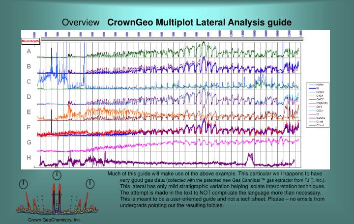
Overview CrownGeo Multiplot Lateral Analysis guide.

E N D
Overview CrownGeo Multiplot Lateral Analysis guide Much of this guide will make use of the above example. This particular well happens to have very good gas data (collected with the patented new Gas Cannibal ™ gas extractor from F.I.T. Inc.). This lateral has only mild stratigraphic variation helping isolate interpretation techniques. The attempt is made in the text to NOT complicate the language more than necessary. This is meant to be a user-oriented guide and not a tech sheet. Please – no emails from undergrads pointing out the resulting foibles. Crown GeoChemistry, Inc.
Description of the plot Multiplot Lateral Analysis guide These tracks can vary from time to time for a particular well, but this is the general format. We’ll discuss each track in following slides. • C1std and C2std • amu51 and C1 • H2/He and H2/C1 • C1 and CO2++ • C1/C4 and C4/C7 • amu51 and C1/(Ar/36) • Sol5 : which is Benz/Nc6 • Gamma : from MWD service In general the data curves are scaled so that each member of each track has the min value at bottom and the max value at top, i.e. as full scale. Sometimes the scales are subtly adjusted so that the overlay of one curve to another can be examined whether or not one curve may have an anomalous high or low “spike”. Historical use of this chart was entirely internal here at Crown and as the charts were internal there was no effort made to unify their appearance – they just ended up however the analyst last had them. Now they are preserved to display this uniform curve set where practical. Crown GeoChemistry, Inc.
Track A : C1std and C2std Multiplot Lateral Analysis guide C1std is the black line and C2std is the green line. These are standardized C1 and C2. Terms like “standardized” and “normalized” can be hard to keep track of – we know, but this set is not that hard to decipher. These are statistical portrayals of the two curves. C1 has a value recorded for every foot of the lateral. These values each are a member of the population of C1 values. If they fell according to this bell curve illustration (illustration from wikipedia.org) then the values at the top center tip of the curve would indicate as 0 (zero) and the values at the edges would be plus3 and minus3 standard deviations. Each methane value is converted in this way for comparison to this data set’s value range. C2 is done the same way. The curves are scaled to overly each other. More on the following plate. Crown GeoChemistry, Inc.
Track A : C1std and C2std Multiplot Lateral Analysis guide Note the red line superimposed over the track. These values climb over the length of the lateral. For light volatile gas like C1 and C2 this happens as length of contributing section is increased. Note the data in the blue circle. These values deviate significantly above the general trend. This data might suggest (all other things being equal) the possibility at the least that this section contains more hydcs and/or can deliver hydcs better than the remainder of the lateral. Note also that there is very good “curve fit” in that the two curves almost perfectly overlie each other. We compare these two hydcs expecting good general agreement except in extremely tight formations. If there is not good fit one should investigate other data to help determine why not. With increasing lateral section the downhole motor can be affected by the loss of horsepower so that more pump pressure is required to turn the bit. The hydrostatic differential will then increase and in longer laterals the upward trending “ramp” can flatten in response to this increase in hydrostatic pressure or, in some cases, even make a dip at the end. Crown GeoChemistry, Inc.
Track B : amu51 and C1 Multiplot Lateral Analysis guide Here we use amu51 which is a sort of a “generic” for large wet hydcs., and plot this against C1 – the lightest smallest hydc. Amu51 is used in this fashion because it is contributed to by several aromatic hydcs but is not the dominant peak for any of them. This “teamwork” contribution effort to that one amu is what makes this amu “generic” for aromatics and that allows us to examine for a concept in a general way even when the signal is too low at the specific parent spots for the contributing species to be examined alone. For a particular lateral the pore pressure, temp, hydc source- migration history, etc – all of these would be expected to not actually have significant variation, and therefore one lateral should have about the same ratio (good overlay) of C1 to C6+aromatics. One would expect these two curves to be capable of being scaled min to max for each such that one curve neatly “fits” to the other as in this diagram. When the curves do not “fit” or co-vary then some thought must be given as to what may be the cause. This is a source-rock shale that has decent perm for a shale so the nearly perfect curve fit is understandable in that this hydc source makes a hydc product that over a few feet does not vary much in component ratios and/or concentrations. In some cases there would be much more variation – as in the following plate Crown GeoChemistry, Inc.
Track B : amu51 and C1 Multiplot Lateral Analysis guide These insets are from a different well than the chart in the prior plate. Note the red “ramp” line superimposed over the chart below. The amu51 values appreciate over lateral length as expected, but the C1 values under-perform vs. amu51 for the deeper portion (black circled inset) of this chart. Why methane does not have the expected value range should then be examined for when making an analysis for this well. Crown GeoChemistry, Inc.
Arrival to source rock Track C : H2/He and H2/C1 Multiplot Lateral Analysis guide Green line is H2/He and the H2/C1 is the blue. The analysis input from these is to examine the behavior of light gas components that have different reasons to be present. Helium and methane are both expected to be gas phase and there should be near-perfect equilibration of the two within each compartment. Existence of variance among these three can be suggestive of several things including compartmental distinction. Hydrogen though is an extremely reactive thing – it can simply interact with too many things to name , including even mud chemistry. H2 then could be used to endorse a concept derived independently but be cautious of allowing H2 to alone either indicate or counter-indicate a concept. Sometimes one of these curves might be replaced by He/C1. Crown GeoChemistry, Inc.
Track D : C1 and CO2 Multiplot Lateral Analysis guide Methane and CO2 are two of the most abundant formation gases measured. These curves are used to evaluate their distributions. Changes in distribution equilibrium can indicate compartmentalization and/or compositional change. Generally we will display CO2++ as this peak has less interference from higher molecular hydcs.. These should co-vary within any given charge compartment and this can be useful when looking for endorsement for compartmental boundary decisions. These should both trend higher over the lengthening lateral, and off-ratio “spikes” might suggest points to examine further for compartmental and structural changes, including faulting and/or secondary fracturing. CO2 is independently interesting to notice in some cases, and the occurrence of CO2 without hydcs or hydcs without CO2 can sometimes be instructive. The mild skew from C1 stronger early to CO2ish later which is indicated by our example data seems inconsequential. Methane here is the duplicate of Track B. This is linear scaled data and it should ramp up more or less evenly across the lateral. The anomalous center section stands out in this plot for that reason, as in the Tracks A and B plots. Crown GeoChemistry, Inc.
Track E : C1/C4 and C4/C7 Multiplot Lateral Analysis guide These two examples are from two different types of hydc environment, and you can see this in the data. Note on the top strip that the tan line (C1/C4) starts early in the lateral with high values which then simply drift down along the lateral. The wetter component of that ratio is C4 which is at nominal values early in the lateral. The area is in fact a notably mature (dry gas) region. After enough hole is opened to allow some accumulation to the system for the scant amounts of the wetter hydcs the ratios change – brown trends up and tan trends down – both because of the relative absence geologically of anything much past Propane. In the other track (below) note that the approximate range for each ratio is similar, so the curve fit in the overlay is of the two is better. Note also that in much of the center of this portion of the lateral the C1/C4 is relatively high. This is a hydrocarbon-drier profile and was in evidence in the other multiplot tracks for that well. So: The top Track E example is not much actual use analytically, and the bottom Track E example suggests the possibility of a distinct feature in that center data portion. Crown GeoChemistry, Inc.
Out-flow Point Track F : amu51 and C1/(Ar/36) Multiplot Lateral Analysis guide This one is actually a bit complex in one sense – but what matters more than that a user can repeat back the entire theory really is that he/she might understand some use of the data. This one is a QC track. The red data line is related to air at low values and to geology at higher values. Remember this sample well is relatively hydc-dry and the hydcs are also approximately evenly distributed thus the nearly perfect overlay or “curve fit” after the point flagged here as the “Out-flow Point”. This is where the hydc amounts being made available to the sample stream through the extraction process is SURPLUS to the amount actually being sampled and the surplus vents OUT of the extractor as exhaust. Prior to this point more sample was being drawn than the hydc count actually extracted and the difference was made up by air flowing IN through that same vent. Compartmental indications based on changes before and after this point and comparisons of data either side of the point may be made but this should be done cautiously. This amu51 data (blue line) is perfectly duplicated in Track B Sample available for extraction is low and supplemented with air inflow at extractor vent Sample is more than sufficient and surplus will be vented out at extractor. Crown GeoChemistry, Inc.
Track G: Sol5 (Benz/nC6)Multiplot Lateral Analysis guide This is very useful in shale laterals and can also be quite useful in other environments. The data should trend higher over lengthening lateral. The principle is that the two hydcs being compared are both about evenly distributed locally in a shale lateral. One , Benzene, is more prone to stay bound (in solution) to the mud system. They both are soluble but one just behaves as if a lot more so. Benz then accumulates to a higher ratio across the section as the other (nC6) frees itself more readily from the mud. Trips and lengthy downtimes do allow the Benz to dissipate over the still mud system and produce a “trip affect” aberration one should watch for. Note in the page-bottom reprint of the same track that the early portion of the well has a steeper “ramp” effect and then later the effect is much more flat. This is apparently the point at which the Benz solubility is reached and surplus amounts aerate more readily. This effect is most often less pronounced than in this well, supporting the decision made elsewhere that this particular point is about at a compartmental boundary. This data can be useful to gauge whether diminished concentrations of lighter species seem to have been sampled correctly. If this data changes (say to half value) and the lighter species also drops to half value then we should investigate sample quality. Alternatively say this one stays put and CO2 does as well, but methane drops; then we might more confidently presume an actual geologic event. This curve should be broadly similar to amu51. Crown GeoChemistry, Inc.
Track F : Gamma (MWD) Multiplot Lateral Analysis guide Data is provided by MWD vendor and is presented here as an analytical tool and as a convenience when this data is compared to other data. Crown GeoChemistry, Inc.