Download
1 / 55
550 likes | 951 Vues
aerosol climatology. S. Kinne and colleagues MPI-Meteorology with support by AeroCom and AERONET. overview. aerosol in (global) climate modeling (tropospheric) aerosol climatology concept column optical properties altitude distribution changes in time link to clouds

E N D
aerosol climatology S. Kinne and colleagues MPI-Meteorology with support by AeroCom and AERONET
overview • aerosol in (global) climate modeling • (tropospheric) aerosol climatology • concept • column optical properties • altitude distribution • changes in time • link to clouds • some applications • further improvements
aerosols ! • aerosol (‘small atmos.particles’) • many sources • short lifetime • diff. magnitudes in size • changing over time • aerosol clouds • aerosol chemistry • aerosol biosphere • aerosol aerosol highly variable in space and time ! rapid atmospheric ‘cycling’ ocean industry cities forest desert volcano
aerosols ? • the radiation budget is modulated by clouds • so, what is all the fuss about aerosol ? • aerosol has a role in cloud formations • many clouds exist because of avail. aerosols • aerosol has an anthropogenic component • the impact on climate is highly uncertain and at times speculative (for indirect effects)
complex aerosol modules • they do exist - even in Hamburg ECHAM/HAM • they are useful … but often too expensive size optically active and relevant sizes
simplifications ? • simplified methods have been tried in the past • ignore aerosol • compensate with a radiation correction • simplify by ignoring fine-mode absorption • improve on the Tanre-scheme used in ECHAM IPCC 4AR simulations • a highly absorbing dust bubble over Africa • lack in seasonal feature (e.g. biomass) • now better simplifications are possible • matured complex aerosol module output • improved obs. constrains by remote sensing
new aero climatology goal • provide a simplified aerosol representation in global models for rapid estimates on aerosol direct & indirect effects on the radiation budget • establish aerosol optical properties (as they required for atmospheric radiative transfer) at sufficient resolution … in order to resolve regional variability and seasonality • whenever possible, tie climatology data to (quality) observations • establish via CCN (cloud condensation nuclei) or IN (ice nuclei) links to cloud properties
data sources • the available observables • ground based in-situ samples • satellite guesses • sun-/sky- photometry • the modeling world • data-constrained simulations • ensemble output
ground samples ? • issues • ground composition is not that of the column • samples are usually heated (less or no water) • monthly statistics example size absorption up quartile median low quartile
satellite data ? • issues • ancillary data needed • indirect reflection info requires information on aerosol absorption (usually assumed) and reflection contribution by other sources (such as surface or clouds) at high accurcay • limited information content • only AOD is retrieved and via AOD spectral dependency some information on size • limited coverage • land?, not with clouds, daytime, not polar, … • positives • spatial distribution statistics
seasonal AOD by satellites combining MODIS, MISR, AVHRR data
ground-based sun-photometry • advantages • direct AOD measurements • AOD and fine-mode AOD • other aerosol properties with sky-radiance data • size distribution (0.05mm < size bins < 15 mm) • single scatt. albedo (noise issue at low AOD) • issues • local … may fail to represent its region • daytime and cloud-free ‘bias’
global modeling • advantages • complete consistent (no data-gaps) • issues • as good as assumptions or the ‘tuning’ AERONET modeling
climatology concept • merge • quality statistics of AERONET • onto • consistent background statistics by global modeling • NO satellite • NO grd in-situ AERONET modeling
aerosol climatology • resolution and data content • processing steps • essential properties • temporal variations • link to clouds • first applications • further improvements
climatology products • global monthly 1x1 lat-lon maps • fine mode (radius < 0.5mm) properties • column AOD, SSA, g (… for each l) • altitude distribution • anthropogenic AOD fraction (1850 till 2100) • pre-industrial AOD fraction • coarse mode (radius > 0.5mm) properties • column AOD, SSA, g (… for each l) • altitude distribution • cloud relevant properties • CCN concentration (kappa approach) • IN concentration (coarse mode dust)
climatology details / steps • define global monthly maps of mid-visible aerosol column prop (AOD, SSA & Ang) • spread data spectrally to define AOD, SSA & g needed for radiative transfer simulations • add altitude information using active remote sensing from space and/or modeling • account for decadal (anthrop.) change using scaling data from aerosol component modeling • establish a (needed) link to cloud properties by extracting associated CCN and IN
column optical properties • concept combine • for mid-visible aerosol properties (0.55 mm) • for monthly (multi-annual) data • for a (1ox1o lon/lat) horizontal resolution • consistent and complete maps from modeling • use AeroCom (15 model ensemble) median composite to remove any extreme behavior • quality data by sun-/sky-photometry networks • data of ~400 AERONET and ~10 Skynet sites
the merging • combine point data on regular grid (1ox1o lon/lat) • extend spatial influence of identified sites with better regional representation • spatially spread valid grid ratios and combine • decaying over +/- 180 (lon) and +/- 45 (lat) • apply ratio field values (A) at site domains with distance decaying weights (B) corr. factors example: correction to model suggested AOD A B A*B ratio field site weight correction factor
merging results model merged AERONET 0.55mm • AOD • SSA • Ang other .. fine-mode anthropogenic fraction kappa dust size
spectral extension (1) • concept • split AOD contribution by small & large sizes • fine-mode size (radii < 0.5um) • coarse-mode size (radii > 0.5um) • apply the Angstrom for total aerosol … with • pre-defined fine-mode Angstrom at function of ‘low clouds’: Ang,f = [1.6 moist … 2.2 dry] • fixed coarse-mode Angstrom: Ang,c = 0.0 • coarse mode (spectr. dep. properties) prescribed • apply the single-scatt. albedo for total aerosol • sea-salt (re=2.5mm / no vis. absorption: SSA = 1.0) • dust (re=1.5, 2.5, 4.5, 6.5, 10mm / SSA =.97, .95, .92, .89, .86
spectral extension (2) • concept • fine-mode spectral dependence by property • only adjustments for solar spectrum needed • AOD spectral dependence is defined by the fine-mode Angstrom parameter [1.6-2.2] range • SSA spectral dependence considers lower values in the near-IR (Rayleigh scattering limit) • asymmetry-factor and its spectral dependence is linked with fine mode Angstrom parameter (sharing common information on aerosol size) g = 0.72 - 0.14*Ang,f *sqrt[l(mm) -0.25] g,min=0.1
spectral samples – annual avg maps g AOD SSA • UV 0.4mm • VIS 0.55mm • n-IR 1.0mm • IR 10mm
altitude distribution • concept … tied to the mid-visible AOD • define altitude distribution for total aerosol • use CALIPSO (vers.2) multi-annual statistics or use ECHAM5 / HAM simulation data • define altitude distribution separately for fine-mode and for coarse-mode aerosol • use ECHAM5 / HAM simulation data • pre-defined layer boundaries 0 - 0.5 - 1.0 - 1.5 - 2.0 - 2.5 - 3.0 - 3.5 - 4.0 - 4.5 - 5 - 6 - 7 - 8 - 9 - 10 - 11 - 12 - 13 (- 15 - 20) km (if surface height > 0.5km less atmos. layers)
total AOD (550nm) by layer ECHAM 5 / HAM CALIPSO vers.2
temporal change • concept • assume that the coarse mode is all natural • assume that the coarse mode does NOT change with time • assume that the pre-industrial fine-mode aerosol fraction does NOT change with time • the only aerosol to change over time is the anthropogenic fraction of the fine-mode (which is by definition zero before 1850)
from the past – from 1860 • concept • use results ECHAM/HAM simulations with NIES historic emissions • aggregate simulated fine-mode monthly AOD patterns in 10 year steps for local monthly decadal trends • linearly interpolate between 10 year steps to get data for individual years • (at this stage) only changes to AOD are allowed … no changes to composition • could be an issues as there was a higher BC before WWII and a higher sulfate fraction after WWII
into the future – until 2100 • concept • simulate with ECHAM/HAM AOD pattern changes by modifying suggested future emissions according to • RCP 2.6 IPCC% scenario • RCP 4.5 IPCC 5 scenario • RCP 8.5 IPCC 5 scenario • simulate changes for sulfate and carbon emissions stratified by selected regions • quantify the associated changes to fine-mode AOD pattern • sum impacts from all regions
link to clouds • aerosol provide CCN and IN to clouds • changes to aerosol concentration can modify cloud properties and the hydrological cycle • critical parameters are • aerosol concentration from climatology • aerosol composition from modeling • super-saturation • temperature
define concentrations • aerosol concentrations …are defined by the AOD vertical distribution and assumed log-normal size-distributions • coarse-mode log-normal properties for sea-salt or dust are prescribed (see above) • fine-mode log-normal width is fixed (std.dev 1.8) and the mode radius is linked to the Angstrom of the fine-mode (which depends on low cloud cover) • larger aerosol radii at moister conditions • smaller aerosol radii at drier conditions
define CCN / IN • all coarse mode particles are CCN … plus • a fraction of fine-mode particles are CCN • for fine-mode concentrations: • a critical cut-off size is determined as function • super-saturation • kappa (‘humidification’) - maps are based on ECHAM/HAM simulations for fine-mode AOD • kappa weights: SS =1.0, SU =0.6, OC =0.1, DU/BC =0) • only sizes larger that the cut-off are considered as fine-mode CCN • coarse mode dust particles are IN
critical fine-mode radius 1km 3km 8km • SS 0.1% • SS 0.2% • SS 0.4% • SS 1.0%
critical fine-mode radius natural CCN anthrop.CCN (dust) IN • SS 0.1% • SS 0.2% • SS 0.4% • SS 1.0%
applications • aerosol direct forcing • in global numbers (vs +2.8 W/m2 by greenhouse) • global direct forcing pattern (highly uneven) • strong seasonality (snow, clouds, aerosol type) • sensitivity to input (define uncertainty range) • temporal change (explore climate sensitivity) • CCN application • first tests for impacts on clouds
direct effects by the numbers • global averages for direct radiative forcing • - 0.5 W/m2 anthropogenic at ToA all-sky • + 0.3 W/m2 for anthropogenic BC • compare to +2.8 W/m2 by greenhouse gases • - 1.1 W/m2 anthropogenic at ToA clear-sky • - 4.7 W/m2 solar at ToA clear-sky • as seen by satellite sensors • - 8.6 W/m2 solar at surface clear-sky • as seen by ground flux radiometers
direct forcing – global patterns solar + IR solar anthrop. solar • clear ToA • clear surface • all-sky ToA • all-sky surface ‘seen’ by satellite ‘seen’ by ground flux-radiometer climate signal coolingwarming
direct forcing – seasonality coolingwarming
direct forcing - sensitivity tests • ToA all-sky forcing uncertainty • examine impact by changing individual prop. to aerosol or environment • +/- 0.3 W/m2 no AERONET lower low clouds AOD uncertainty higher low clouds AOD by satellite SSA uncertainty fine-mode = anthropogen higher surf. albedo g uncertainty higher max. for fine mode absorption higher surf. albedo 25% more absorption
anthrop. direct forcing in time • changing pattern • 1940: -.16 W/m2 • 1945: -.17 W/m2 • 1950: -.19 W/m2 • 1955: -.21 W/m2 • 1960: -.24 W/m2 • 1965: -.27 W/m2 • 1970: -.31 W/m2 • 1975: -.35 W/m2 • 1980: -.38 W/m2 • 1985: -.41 W/m2 • 1990: -.43 W/m2 • 1995: -.44 W/m2 strongest increase
CCN – climatology in use • CCN /ccm3 at 1km 0.1% super-saturation • liquid water path comp. • stronger aerosol indirect effect with the climatology climatology ECHAM5.5/HAM by U.Lohmann ETHZ
future improvements • update AOD vertical distribution with CALIPSO version 3 data (multi-annual averages) • include compositional change over time for anthropogenic aerosol (BC vs sulfate content) • allow responses to relative humidity changes in the boundary layer • explore smarter ways for data merging of trusted point data onto background data • allow natural aerosol (sea-salt and dust) to vary according to met-data and/or to soil-data
data access ftp ftp-projects.zmaw.de • cd aerocom/climatology/2010/yr2000 • look at ‘README_nc’ • ss-properties for the 14 solar-bands of ECHAM6 • g30_sol.nc total aerosol (yr 2000) • g30_coa.nc coarse mode aerosol • g30_pre.nc fine-mode pre-industrial (yr 1850) • g30_ant.nc fine-mode anthropogenic (yr 2000) • ss-properties for the 16 IR-bands of ECHAM6 • g30_fir.nc total (=coarse mode) aerosol • CCN and IN fields • g_CCN_km20.nc for supersat. of 0.1, 0.2, 0.4 and 1% • anthrop. CCN is changing along with anthrop. AOD year 2000 properties
data access ftp ftp-projects.zmaw.de • cd aerocom/climatology/2010/ant_historic • based on decadal change by ECHAM/HAM simulations for fine mode aerosol with NIES historic emissions • aeropt_kinne_550nm_fin_anthropAOD_yyyy.nc • simulations by Silvia Kloster, prep. by Declan O’Donnell • cd aerocom/climatology/2010/ant_future • based on sulfate and carbon emission related regional changes to fine-mode AOD patterns with ECHAM/HAM for IPCC RCP 2.6, RCP 4.5 and RCP 8.5 scenarios till 2100 • aeropt_kinne_550nm_fin_anthropAOD_rcp??_yyyy.nc • simulations by Kai Zhang, concepts by Hauke and Bjorn anthropogenic change
data access ftp ftp-projects.zmaw.de altitude • cd aerocom/climatology/2010/altitude • based on CALIPSO version2 multi-annual data • fine/coarse mode altitude differences via ECHAM/HAM • calipso_fc.nc • CALIPSO data via Dave Winker (NASA_LaRC) • ECHAM/HAM altitude data from Philip Stier • cd aerocom/climatology/2010/ccn_historic • applying anthropogenic change to CCN concentrations • CCN_1km_yyyy.nc at 1km above ground • CCN_3km_yyyy.nc at 3km altitude • CCN_8km_yyyy.nc at 8km altitude
extra plots • mid-visible aerosol ss-properties • current anthropogenic AOD … by month • solar spectral ant aerosol properties variations • vertical spread of fine mode AOD by ECHAM • vert. spread of coarse mode AOD by ECHAM