Download
1 / 15
150 likes | 293 Vues
Exponential Functions. Lesson 5.1. You have used sequences and recursive rules to model geometric growth or decay of money, populations, and other quantities. Recursive formulas generate only discrete values. Growth and decay happen continuously.

E N D
Exponential Functions Lesson 5.1
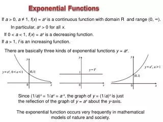
You have used sequences and recursive rules to model geometric growth or decay of money, populations, and other quantities. • Recursive formulas generate only discrete values. • Growth and decay happen continuously. • We will study explicit formulas for these patterns, which will allow you to model situations involving continuous growth and decay, or to find discrete points without using recursion.
Radioactive Decay • This investigation will simulate radioactive decay. • Each person will need a standard six-sided die. • Each standing person represents a radioactive atom in a sample. • The people who sit down at each stage represent the atoms that underwent radioactive decay.
Follow these steps • Collect data in the form (stage, number standing). • All members of the class should stand up, except for the recorder. The recorder counts and records the number standing at each stage. • Each standing person rolls a die, and anyone who gets a 1 sits down. • Wait for the recorder to count and record the number of people standing. • Repeat the last two steps until fewer than three students are standing.
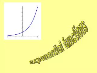
Graph your data. The graph should remind you of the sequence graphs you studied in Chapter 1. • What type of sequence does this resemble? • Identify uo and the common ratio, r, for your sequence. Complete the table below. • Use the values of uo and r to help you write an explicit formula for your data.
0 u0 u1 U0 (r) U0 (r) 1 2 u2 U0 (r)(r) U0 (r)2 3 U0 (r)(r)(r) U0 (r)3 u3 4 u4 U0 (r)(r)(r)(r) U0 (r)4
Graph your explicit formula along with your data. Notice where the value of u0 appears in your equation. Your graph should pass through the original data point (0, u0 ) . Modify your equation so that it passes through (1, u1) , the second data point. (Think about translating the graph horizontally and also changing the starting value.)
Experiment with changing your equation to pass through other data points. • Decide on an equation that you think is the best fit for your data. Write a sentence or two explaining why you chose this equation. • What equation with ratio r would you write that contains the point (6, u6) ?
Example A • Most automobiles depreciate as they get older. • Suppose an automobile that originally costs $14,000 depreciates by one-fifth of its value every year. • What is the value of this automobile after 2 1/2 years? • When is this automobile worth half of its initial value?
To find when the automobile is worth half of its initial value, or 7,000 replace the y with 7000 and solve for x. 7,000= 14,000(1- 0.2)x 0.5= (1- 0.2)x 0.5 =(0.8)x You don’t yet know how to solve for x when x is an exponent, but you can experiment to find an exponent that produces a value close to 0.5. The value of (0.8)3.106 is very close to 0.5. This means that the value of the car is about $7,000, or half of its original value, after 3.106 years (about 3 years 39 days). This is the half-life of the value of the automobile, or the amount of time needed for the value to decrease to half of the original amount.
Example B The functions and are transformations of the parent function . Describe the transformations and sketch the graphs. The graph of g (x) is a vertical dilation of the graph of f (x) by a factor of 1/2. The marked points on the red graph show how the y-values of the corresponding points on the black graph have been multiplied by 1/2 .
Example B The functions and are transformations of the parent function . Describe the transformations and sketch the graphs. The graph of h(x) is a horizontal translation of the graph of f (x). The marked points on the red graph show how the corresponding points on the black graph have been moved right 1 unit.