Download
1 / 32
330 likes | 491 Vues
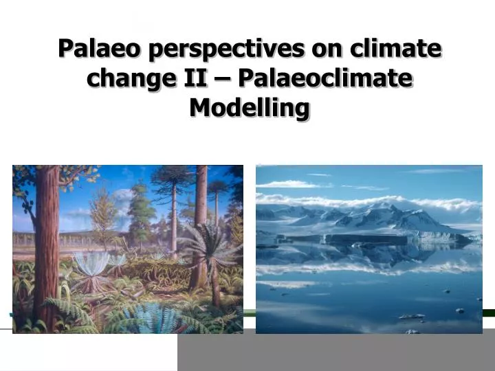
Palaeo perspectives on climate change II – Palaeoclimate Modelling. Content. Introduction to Cenozoic climate change How do we do it & what do we need? – bringing modellers and data collectors together Case studies: A permanent El Niño-like state during the Pliocene?

E N D
Palaeo perspectives on climate change II – Palaeoclimate Modelling
Content • Introduction to Cenozoic climate change • How do we do it & what do we need? • – bringing modellers and data collectors together • Case studies: • A permanent El Niño-like state during the Pliocene? • The role of Polar Ocean Gateways in EAIS development • Can models reproduce Greenhouse ice sheets? • Plus a little surprise.
Climate History
The Future: Data & Models Combine • Limiting Factors: • Available computer power • Model sophistication (resolution etc.) • Small community (“every department needs a pet modeller”) • Language barriers & a lack of communication • A new generation of scientists to act as the interface • A couple of examples what modellers need from the geological community • Ocean temperatures • Land cover “Deep-time perspectives on climate change: marrying the signal from computer models and biological proxies (Eds. M. Williams, A. M. Haywood, J. Gregory and D. Schmidt) The Micropalaeontological Society & the Geological Society of London”
Oceans: Quantitative temperature estimates derived from multi-proxy studies PRISM & MARGO Kucera et al. (2005) QSR Vol. 24, 813-819 H. Dowsett (in-press).
New 3-D Ocean Temperature Reconstructions: multiple equilibrium?
Land Cover: Vegetation and Biomes derived from paleobotanical studies Proxies Data Biomes Pollen Rainforest Translation and Reconstruction Fossil Leaves Grassland • Nearest Living Relatives • Plant functional types • Full Biomisation Savanna Fossil Wood
Paleo-Data Biomes PLIOCENE BIOMES:DATA–MODEL COMPARISON Model Biomes
Case Studies 1. Palaeo ENSO (El Niño Southern Oscillation) • Coupled ocean-atmosphere • phenomena • Involves large scale fluctuations • in a number of oceanic/atmospheric variables (e.g. sea surface temps. • & sea level pressure) • El Niño & La Niña opposite extremes • of ENSO
Strong Gradient No Gradient The Pliocene: a Permanent El Niño-like state? (Wara et al., 2005; Philander & Federov, 2003) Mg/Ca SSTs 0 3 5 Age (Ma)
Can a model reproduce this change? PlioControl ocean temperatures (C) across the Pacific at 0N Difference between PlioceneControl and Pre-Ind (C) 0 400 1000 3000 5000
ENSO rather than permanent El-Niño! Haywood et al. (2007). Paleoceanography
“In search of palaeo-ENSO: significance of changes in the mean state” 1 sample per 10,000 years
Additional Modelling Experiments • Ocean Gateways • Trace Gas Concentrations • Altered Model Parameters
Case Studies 2. Ice-Sheet Initiation (E/O boundary) Marine 180 Antarctic ice-rafted detritus E/O boundary Palaeobotanical Evidence Zachos et al. (2001)
Palaeocene Present Antarctica: from Greenhouse to Ice-house
Ocean Currents
Case Studies 3. Cretaceous Climates & Ice-Sheets Palaeobotanical Evidence Cretaceous forest 120 million years ago on the Antarctic Peninsula. reconstruction based on PhD of Jodie Howe, University of Leeds/BAS, painted by Robert Nichols.
Evidence for large, rapid sea-level changes (Miller et al., 2005) • Evidence for eustatic nature • Pace and magnitude suggest glacial origin. • Suggest moderate-sized ice sheets (5 - 10 × 106 km3 ). • Paced by Milankovitch forcing. • CO2 levels through the Maastrichtian • 2 greenhouse episodes 1000-1400 ppm • But suggestions of CO2 low-points at ~70 and 66 Ma. • (Nordt et al., 2003; Beerling et al., 2002).
How to create a Maastrictian model Change solar output ~0.6% less than present CO2 (and other gases) 4 x pre-industrial (but could be 2x to 8x. Volcanic activity Assume same as today. Change in orbit Same as present, but perform sensitivity simulations Palaeogeography Including sea-level/ orography/ bathymetry/land ice Previous modelling also required prescription of vegetation, and sea surface temperatures (or ocean heat transport) but this is no longer needed.
Maastrictian Orography At climate model resolution. Original palaeogeographies from Paul Markwick
Coupled Ocean-Atmosphere Simulation:Comparison to Oxygen Isotopes Model predicted temperatures approx. 10C at 1000m, 8C at 2000m, and 7C at 3000m c.f. temperatures from 14C to 7C from D’Hondt & Arthur (2002) Paul Pearson's Maastrictian data
Coupled Ocean-Atmosphere Simulation:Comparison to Vertebrate Data Red squares= all crocs, Orange= Dinosaurs, White = Other Vertebrates Model predicted cold month mean shown by 5C contour(red)and 0C(blue) Paul Markwick's database
2xCO2 - ~ 2 x 10⁶ km3 ice Ice Sheets in a Greenhouse World • Suite of HadCM3 derived palaeoclimates • 2, 4, and 6 x CO2 • Further runs being carried out including 1 x CO2 • Comparison against climate proxy database • Climate then used to drive a BAS ice-sheet model. 2xCO2 4xCO2 + favourable orbit
Case Studies Constraining Earth System Sensitivity “Equilibrium climate sensitivity refers to the equilibrium change in global mean surface temperature following a doubling of the atmospheric (equivalent) CO2 concentration (Charney sensitivity)”. Estimates based around components of the Earth system that respond quickly (atmosphere, surface ocean) and neglects feedbacks linked to changing deep ocean circulation, vegetation distribution and ice sheets, which can be referred to as Earth System Sensitivity. IPCC 2007: 2 to 4.5°C. Best estimate is 3°C. Is this supported by palaeoclimatology
What do you need? • Interval of time warmer than the pre-industrial • Caused, at least in part, by higher atmospheric CO2 • Orography as close to modern as possible • Evolutionary effects at a minimum • Well constrained geologically • Mid-Holocene? • Last Glacial Maximum? • Any interval in the Pleistocene (last 2 million years) • Cretaceous or Eocene super greenhouse events? • The Pliocene?
Climate evolution - the last 5 million years From Rainer Zahn Legacy of ODP.
How can we do it? We need a model!
The Numbers Please IPCC Climate Sensitivity = 3°C Estimate of Earth System Sensitivity = 4.7°C ESS 60% larger than traditional CS!!! “This work argues that the climate change associated with a doubling of CO2 is likely to be significantly larger than has traditionally been estimated. Calculations which have estimated emissions reductions/capping needed to avert dangerous climate change may need to be re-addressed”.