Download
1 / 33
340 likes | 476 Vues
Engineering 45. Imperfections In Solids. Bruce Mayer, PE Licensed Electrical & Mechanical Engineer BMayer@ChabotCollege.edu. Learning Goals. Learn The Forms of Defects in Solids Use metals as Prototypical Example How the number and type of defects Can be varied and controlled

E N D
Engineering 45 ImperfectionsIn Solids Bruce Mayer, PE Licensed Electrical & Mechanical EngineerBMayer@ChabotCollege.edu
Learning Goals • Learn The Forms of Defects in Solids • Use metals as Prototypical Example • How the number and type of defects Can be varied and controlled • How defects affect material properties • Determine if “Defects” or “Flaws” are • Desirable • UNdesirable
Classes of Imperfections • POINT Defects • Atomic Vacancies • Interstitial Atoms • Substitutional Atoms • LINE Defects • (Plane Edge) Dislocations • Area Defects • Grain Boundaries • Usually 3-D
Point Defects • Vacancy MISSING atom at Lattice Site Vacancy distortion of planes self- interstitial distortion of planes • Self-Interstitial “Extra” Atom “Squeezed” into the Lattice Structure
Point Defect Concentration • Equilibrium Defect Concentration Varies With Temperature; e.g., for Vacancies: Activation energy No. of defects æ ö - N Q ç ÷ v v = ç ÷ exp No. of potential è ø N k T defect sites. Temperature Boltzmann's constant • k = • 1.38x10⁻²³ J/at-K • 8.62x10⁻⁵ eV/at-K • N Every Lattice Site is a Potential Vacancy
Measure Activation Energy • Recall The Defect Density Eqn • Take the ln of Eqn • This of the form • This form of a Negative Exponential is called an Arrhenius Relation • Svante Arrhenius: 1859-1927, Chem Nobel 1903
N N v v N N Measure Activation Energy cont • By ENGR25 method of Function Discovery • Meausure ND/N vs T slope ln - Q /k v exponential dependence! T 1/ T • RePlot in Linear Form • y = mx + b • Find the Activation Energy from the Slope
Vacancy Concentration Exmpl • In Defect Density Rln QD Can Take Two forms • Qv Vacancies • Qi Interstitials • Consider a Qv Case • Copper at 1000 C • Qv = 0.9 eV/at • ACu = 63.5 g/mol • = 8400 kg/cu-m • Find the Vacancy Density • First Find N in units of atoms per cu-m
Vacancy Concentration cont • Since Units Chk: • Now apply the Arrhenius Relation @1000 ºC • 275 ppm Vacancy Rate • At 180C (Pizza Oven) The Vacancy Rate 98 pptr
Low energy electron microscope view of a (110) surface of NiAl. I sland grows/shrinks to maintain equil. vancancy conc. in the bulk. Observing Equil Vacancy Conc 575μm X 575μm Image • Increasing T causes surface island of atoms to grow. • Why? The equil. vacancy conc. increases via atom motion from the • crystal to the surface, where they join the island.
Substitutional alloy (e.g., Cu in Ni) Interstitial alloy (e.g., C in Fe) Point Impurities in Solids • Two outcomes if impurity (B) added to host (A) • Solid solution of B in A (i.e., random dist. of point defects) OR • Solid solution of B in A plus particles of a NEW PHASE (usually for a larger amount of B) • Second phase particle • different composition (chem formula) • often different structure • e.g.; BCC in FCC
W. Hume – Rothery Rule • The Hume–Rothery rule Outlines the Conditions for substitutional solid soln • Δr (atomic radius) < 15% • Proximity in periodic table • i.e., similar electronegativities • Same crystal structure for pure metals • Valency • All else being equal, a metal will have a greater tendency to dissolve a metal of higher valency than one of lower valency
Element Atomic Crystal Electro- Valence Radius Structure nega- (nm) tivity Cu 0.1278 FCC 1.9 +2 C 0.071 H 0.046 O 0.060 Ag 0.1445 FCC 1.9 +1 Al 0.1431 FCC 1.5 +3 Co 0.1253 HCP 1.8 +2 Cr 0.1249 BCC 1.6 +3 Fe 0.1241 BCC 1.8 +2 Ni 0.1246 FCC 1.8 +2 Pd 0.1376 FCC 2.2 +2 Zn 0.1332 HCP 1.6 +2 Imperfections in Solids • Application of Hume–Rothery rules Solid Solutions 1. Would you predictmore Al or Ag to dissolve in Zn? 2. More Zn or Al in Cu?
Element Atomic Crystal Electro- Valence Radius Structure nega- (nm) tivity Cu 0.1278 FCC 1.9 +2 C 0.071 H 0.046 O 0.060 Ag 0.1445 FCC 1.9 +1 Al 0.1431 FCC 1.5 +3 Co 0.1253 HCP 1.8 +2 Cr 0.1249 BCC 1.6 +3 Fe 0.1241 BCC 1.8 +2 Ni 0.1246 FCC 1.8 +2 Pd 0.1376 FCC 2.2 +2 Zn 0.1332 HCP 1.6 +2 Apply Hume – Rothery Rule • Would you predictmore Al or Ag to dissolve in Zn? • Δr → Al (close) • Xtal → Toss Up • ElectronNeg → Al • Valence → Al • More Zn or Al in Cu? • Δr → Zn (by far) • Xtal → Al • ElectronNeg → Zn • Valence → Al
Composition/Concentration • Composition Amount of impurity/solute (B) and host/solvent (A) in the SYSTEM. • Two Forms • Weight-% • Atom/Mol % • Where • mJ = mass of constituent “J” • Where • nmJ = mols of constituent “J” • Convert Between Forms Using AJ
Linear Defects → Dislocations • Edge dislocation: extra half-plane of atoms • linear defect • moves in response to shear stress and results in bulk atomic movement (Ch 7,8) • cause of slip between crystal planes when they move
Movement of Edge Dislocations • Dislocations Move Thru the Crystal in Response to Shear Force • Results in Net atomic Movement or DEFORMATION
Dislocation motion requires the successive bumping of a half plane of atoms (from left to right here). Bonds across the slipping planes are broken and remade in succession Motion of Edge Dislocation
Carpet Movement Analogy • Moving a Large Carpet All At Once Requires MUCH Force (e.g.; a ForkLift Truck) • Using a DISLOCATION Greatly Facilitates the Move Dislocation
Carpet Dislocation • Continue to Slide Dislocation with little effort to the End of the Crystal • Note Net Movement at Far End Dislocation
deformed steel (40,000X) Ti alloy (51,500X) Dislocations • First PREDICTED as defects in crystals since theoretical strength calculations (due to multibond breaking) were far too high as compared to experiments • later invention of the Transmission Electron Microscope (TEM) PROVED their Existence
Interfacial Defects • 2D, Sheet-like Defects are Termed as Interfacial • Some Macro-Scale Examples • Solid Surfaces (Edges) • Bonds of Surface Atoms are NOT Satisfied • Source of “Surface Energy” in Units of J/sq-m • Stacking Faults – When atom-Plane Stacking Pattern is Not as Expected • Phase Boundaries – InterFace Between Different Xtal Structures
Crack Along GB Interface Def. → Grain Boundaries • Grain Boundaries • are Boundaries BETWEEN crystals • Produced by the solidification process, for example • Have a Change In Crystal Orientation across them • IMPEDE dislocation motion • Generally Weaker that the Native Xtal • Typically Reduce Material Strength thru Grain-Boundary Tearing
Schematic Representation Note GB Angles ~ 8cm Area Defects: Grain Boundaries • Metal Ingot: GB’s Follow Solidification Path
Optical Microscopy • Since Most Solid Materials are Opaque, MicroScope Uses REFLECTED Light • These METALLOGRAHPIC MScopes do NOT have a CONDENSOR Lens
Optical MicroScopy cont • The Resolution, Z • The Magnification, M • Where • Light Wavelength • 550 nm For “White” Light (Green Ctr) • NA Numerical Aperture for the OBJECTIVE Lens • 0.9 for a Very High Quality Lens • Typical Values • Z 375 nm • Objects Smaller than This Cannot be observed • Objects Closer Together than This Cannot Be Separated • Mtrue 200
Optical MicroScopy cont.2 • Sample Preparation • grind and polish surface until flat and shiny • sometimes use chemical etch • use light microscope • different orientations → different contrast • take photos, do analysis • e.g. Grain Sizing
Optical MicroScopy cont.3 • Grain Boundaries • are imperfections, with high surface energy • are more susceptible to etching; may be revealed as • dark lines due to the change of direction in a polycrystal • ASTM E-112 Grain Size Number, n microscope polished surface surface groove grain boundary • Where • N grain/inch2 Fe-Cr alloy
Electron Microscopy • For much greater resolution, use a BEAM OF ELECTRONS rather that light radiation • Transmission Electron Microscopy (TEM): • VERY high magnifications • contrast from different diffraction conditions • very thin samples needed for transmission • Scanning Electron Microscopy (SEM): • surface scanned, TV-like • depth of field possible
Polymer Atomic Force MicroScopy • AFM is Also called Scanning Probe Microscopy (SPM) • tiny probe with a tinier tip rasters across the surface • topographical map on atomic scale
SEM Photo Scaling • MEMS Hinge ► Find Rectangle Length Lactual 2.91 in-photo 3.02 in-photo
SEM Photo Scaling • Use “ChainLink” Cancellation of Units(c.f. ENGR10) • Thus the Rectangular Connecting Bracket is about 48µm in Length
Olympus DUV Metallurgical Mscope DeepUltravioletMicroscope U-UVF248