Download
1 / 39
390 likes | 496 Vues
DQO Training Course Day 3 Module 20. The EPA 7-Step DQO Process. Step 7 - Optimize Sample Design DQO Case Study. Presenter: Sebastian Tindall. 45 minutes. Step 7- Optimize Sample Design. Go back to Steps 1- 6 and revisit decisions. Optimal Sample Design. No. Yes.

E N D
DQO Training Course Day 3Module 20 The EPA 7-Step DQO Process Step 7 - Optimize Sample DesignDQO Case Study Presenter: Sebastian Tindall 45 minutes
Step 7- Optimize Sample Design Go back to Steps 1- 6 and revisit decisions. Optimal Sample Design No Yes Information INActionsInformation OUT From Previous Step To Next Step Review DQO outputs from Steps 1-6 to be sure they are internally consistent Decision Error Tolerances Develop alternative sample designs For each design option, select needed mathematical expressions Gray Region Select the optimal sample size that satisfies the DQOs for each data collection design option Check if number of samples exceeds project resource constraints
Terminal Objective To be able to use the output from the previous DQO Process steps to select sampling and analysis designs and understand design alternatives presented to you for a specific project
Sampling Approaches • Sampling Approach 1 • Simple Random • Traditional fixed laboratory analyses • Sampling Approach 2 • Systematic Grid • Field analytical measurements • Computer simulations • Dynamic work plan
Design Approaches Approach 1 Collect samples using Simple Random design. Use predominantly fixed traditional laboratory analyses and specify the method specific details at the beginning of DQO and do not change measurement objectives as more information is obtained
Plan View Former Pad Location Buffer Zone 0 50 100 150 ft 0 15 30 46 m Runoff Zone Approach 1 Sample Design
“Normal” Approach Due to using only five samples for initial distribution assessment, one cannot infer a ‘normal’ frequency distribution Reject the ‘Normal’ Approach and Examine ‘Non-Normal’ or ‘Skewed’ Approach
Pb, U, TPH (DRO/GRO) • Because there were multiple COPCs with varied standard deviations, action limits and LBGRs, separate tables for varying alpha, beta, and (LBGR) delta were calculated • For the U, Pb, and TPH, the largest number of samples for a given alpha, beta and delta are presented in the following table
Aroclor 1260: Non-Parametric Test • For PCBs, the Aroclor 1260 has the greatest variance and using the standard deviation results in a wide gray region • The following table presents the variation of alpha, beta and deltas for Aroclor 1260
Approach 1 Sampling Design (cont) Sub-surface Soils S&A Costs
Approach 1 Sampling Design (cont.) Surface Soils
Approach 1 Sampling Design (cont.) Sub-surface Soils
Approach 1 Based Sampling Design • Design for Pb, U, TPH • Alpha = 0.05; Beta = 0.2; Delta = total error • The decision makers agreed on collection of 9 surface samples for Pb, U and TPH (GRO & DRO) from each of the two surface strata, for a total of 18 samples using a stratified random design • For the sub-surface, nine borings/probes will be collected from each of the two subsurface stratum at random locations, collected at a random depth down to 10 feet, to assess migration through the vadose zone, for a total of 18 samples • Design for PCBs • Alpha = 0.05; Beta = 0.20; Delta = 0.50 (50% of the AL) • The decision makers agreed on collection of 24 surface samples from each of the two surface strata; total of 48 samples using a stratified random design • For the sub-surface, 24 borings/probes will be collected from each of the two subsurface stratum at random locations, collected at a random depth down to 10 feet for a total of 48 samples (2 X 24)
Plan View Former Pad Location Buffer Zone 0 50 100 150 ft 0 15 30 46 m Runoff Zone Approach 1 Sample Locations(Surface Strata)
Remediation Costs* *Does not include layback area
Approach 1 Based Sampling Design • Compare Approach 1 costs versus remediation costs • Approach 1 S&A costs • $11,700 (Pb, U, TPH) + $21,600 (PCBs) = $33,300 • Remediation costs • Cost to remediate surface soil under footprint of pad and buffer area: $204,200 • Cost to remediate subsurface soil under footprint of pad and buffer area: $3,881,400
Design Approaches Approach 2: Dynamic Work Plan (DWP) & Field Analytical Methods (FAMs) • Manage uncertainty by increasing sample density by using field analytical measurements • Manage uncertainty by including RCRA metals as COPCs • Use DWP to allow more field decisions to meet the measurement objectives and allow the objectives to be refined in the field using DWP
Approach 2 Sampling Design • Phase 1: Pb, U, TPH, PCBs • Perform field analysis of the four strata on-site using XRF (RCRA metals & U), on-site GC (TPH), and Immunoassay (PCBs) methods. Take into account the chance of false positives at the low detection levels • This will produce a worse-case frequency distributions and variance for each COPC that will be used to select the proper statistical method and then calculate the number of confirmatory samples for laboratory analysis for the surface and below grade strata
Approach 2 Sampling Design (cont.) • Phase 1: Metals, TPH, PCBs • Provide detailed SOPs for performance of FAMs: XRF, GC, & Immunoassay analysis • Divide both surface strata into triangular grids • Use systematic sampling, w/random start (RS), to locate sample points; sample in center of each grid • Pad & Run-off zone • CSM expects contamination more likely here • 10 ft equilateral triangle: 43.35 ft2 • Pad + Run-off zone = 12,272 ft2 • 283 sample points • Buffer area: • Also 283 sample points • CSM expects contamination less likely here • Thus, grid triangle has larger area
Approach 2 Sampling Design (cont.) • Phase 1: Pb, U, TPH, PCBs • Sub-surface strata: Pad & Run-off zone • Use Direct Push Technology (DPT) to collect • Push at all surface sample points > ALs • Minimum sample locations: 40 (+ 10 >ALs) = ~50 • Collect sub-surface samples at 3-7-10 feet • 50 X 3 = 150 sub-surface samples in this strata • Use systematic sampling, w/random start (RS), to locate sample points • Buffer area • CSM expects contamination less likely here • Thus, fewer sample points • Same >ALs rationale as above • 50 X 3 = 150 sub-surface samples in Buffer area • Use systematic sampling, w/RS, to locate sample points
N Stratified Systematic Grid with Random Start(Surface Strata) Runoff Zone (Stratum 1) Footprint of Concrete Pad (Stratum 1) Buffer Zone (Stratum 2) Not to scale Triangles will be adjusted according to Step 7 design
Approach 2 Sampling Design (cont.) • Phase 2: Pb, U, TPH, PCBs • Evaluate the FAM results, calculate variance and construct FDs for each COPC • Using Monte Carlo method, sample the worst case distribution and evaluate the alpha, beta and delta values and resulting n based on the XRF, on-site GC, and Immunoassay data and select a value (worst case) for n to confirm the FAM data, using traditional laboratory analysis for each of the four strata • For this Case Study, we will assume that number came out to be 9 per strata or 36 confirmatory lab samples
FAM ProcedureSW-846, Draft Update IVAMethod 6200 Field portable x-ray fluorescence spectrometry for the determination of elemental concentrations in soil and sediment
FAM ProcedureSW-846, Draft Update IIIMethod 4020 Screening for polychlorinated biphenyls by immunoassay
FAM Procedure for GROSW-846, Draft Update IIIPreparation Method 5030 or 5035(purge and trap methods)Followed by Analysis Method 8015 B Non-halogenated organics using GC/FID
FAM Procedure for DROSW-846, Draft Update III One of Following Extraction Methods: • 3540 (soxhlet), • 3541(auto-soxhlet), • 3550 (ultrasonic), or • 3560 (super critical fluid) Followed by Analysis Method 8015 B: • Non-halogenated organics using GC/FID
Approach 2 Sampling Design (cont)Sub-surface Soils SC&SA Costs
Approach 2 Sampling Design (cont.) • Evaluate costs of Approach 2 vs. remediation costs • Sampling and analysis (S&A) costs $143,624 • Original budget for S&A $45,000 • Remediation cost • Cost to remediate surface soil under footprint of pad and buffer area: $204,200 • Cost to remediate subsurface soil under footprint of pad and buffer area: $3,881,400
Approach 2 Sampling Design (cont.) • Remediation Costs: • Surface - $204,200 • Sub-surface - $3,881,400
QC and Analysis DetailsUsed in All Approaches • Measure gasoline & diesel range organics (GRO/DRO) • Ship & process all samples in one batch to decrease cost. • QC defined per SW 846 [1 MS/MSD, 1 method blank, 1 equipment blank (if equipment is reused), 1 trip blank for GRO only]. • Cool GRO/DRO to 4°C, 2°C. • QAP written and approved before implementation.
End of Module 20 Thank you Questions?