Download

1 / 39
400 likes | 654 Vues
Blend Times in Stirred Tanks Reacting Flows - Lecture 9. Instructor: André Bakker. © Andr é Bakker (2006). Evaluation of mixing performance. Methods to evaluate mixing performance: Characterization of homogeneity. Blending time. General methods to characterize homogeneity:

E N D
Blend Times in Stirred Tanks Reacting Flows - Lecture 9 Instructor: André Bakker © AndréBakker (2006)
Evaluation of mixing performance • Methods to evaluate mixing performance: • Characterization of homogeneity. • Blending time. • General methods to characterize homogeneity: • Visual uniformity. • Quantitative change in local concentration as a function of time. • Review instantaneous statistics about the spatial distribution of the species. • Average concentration • Minimum and maximum • Standard deviation in the concentration. • Coefficient of variation CoV = standard deviation/average.
Visual uniformity • Experimentally measure the time it takes to obtain visual uniformity. • Can be done with acid-base additions and a pH indicator. • Offers good comparisons between performance of different mixing systems. • Not a suitable approach for CFD.
Visual uniformity example: glass mixing • Glass exits the glass ovens with variations in temperature and material concentrations. • As a result, when the glass hardens, there will be visual non-uniformities. • So, glass needs to be mixed before it is used. Because of the high-viscosity and temperature, special mixers are used, • Optical quality of glass is still often determined visually.
Quantitative variation in a point • Measuring the tracer concentration as a function of time c(t) in one or more points in the vessel, is a common experimental method. • The mixing time is then the time it takes for the measured concentration c(t) to stay within a certain range of the final concentration c. • Advantage: easy to use in experiments. • Disadvantage: uses only one or a few points in the vessel. • Does not use all information present in a CFD simulation. Concentration 99% mixing time 90% mixing time Time
Blend time calculations with CFD • Transport and mixing of a tracer: • Add tracer to the domain. • Mass fraction of tracer calculated and monitored as a function of time. • Determine blend time based on the mass-fraction field satisfying a pre-specified criterion. • Flow field required can be steady, frozen unsteady or unsteady. • Benefit of CFD: • The full concentration field is known. • Can use more data to determine blend time than what can be measured experimentally using probes. • Main question: what should be the mixing criterion?
CFD analysis for blend time • We will now: • Illustrate the blend time analysis using a 2-D Rushton turbine flow field example. • Tracer added and its transport and mixing calculated. Mass fractions are monitored as a function of time. • Blend time is calculated using different criteria.
Measures of variation • Variations in Y, the mass fraction of tracer, can be measured in several ways. For all measures, greater numbers indicate a greater variation with no upper bound. • Coefficient of variation. Ratio between standard deviation Y and the average <Y>: • Ratio between maximum and minimum mass fractions Ymax/Ymin. • Largest deviation between extremes in the mass fraction and the average: Can also be normalized over <Y>.
t=10s Variation calculation example • Mass fraction data: • Min-max anywhere: 0.0223-0.539 • Min-max from probes: 0.0574-0.272 • Average: 0.0943 • Standard deviation: 0.049 3 • Measures of variation: • Max/min = 0.539/0.0223 = 24.2 (anywhere) • Max/min = 0.272/0.0574 = 4.7 (from probes) • CoV = 0.0493/0.0943 = 0.52 • max = max(0.539-0.0943, 0.0943-0.0223) = 0.44 • max/<Y> = 0.44/0.0943 = 4.7
Variation max/<Y> CoV Ymax/ Ymin max Time (s)
Measures of uniformity - absolute • There is a need to have an absolute measure of uniformity U that is 1 with 1 (or 100%) indicating perfect uniformity. • Ratio between the minimum and maximum mass fractions. • Bounded between 0 and 1. • Based on coefficient of variance CoV: • Not bounded: can be less than 0. • Based on largest deviation from the average: • Conceptually closer to common experimental techniques. • Not bounded: can be less than 0.
Uniformity UCoV= 1-CoV Umin/max U=1-max/<Y> Time (s)
Uniformity • These measures of uniformity: • All indicate perfect uniformity at values of 1. • Are not all bounded between 0 and 1. • Do not take initial conditions into account. • Generally, it is most useful to be able to predict the time it takes to reduce concentration variations by a certain amount. • This is then done by scaling the largest deviation in mass fraction at time t by the largest deviation at time t=0. • E.g. for the example case: • At t=0s, Ymax=1 and <Y>=0.0943 max(t=0) = 0.906. • At t=10s, max(10s) = 0.44 U(10s) = 0.51. • Data are often correlated in terms of number of impeller revolutions, at t=10s and 50RPM, there were 10*RPM/60=8.33 impeller revolutions.
U 99% mixing time 90% mixing time Blend time is then the time it takes to reduce the initial variation by a given percentage. Impeller revolutions
Comparison between systems • Let’s compare two systems with: • The same flow field. • The same spatial distribution of species. • But different initial mass fractions of species. Layer with Ytracer=1 on top of fluid with Ytracer =0. <Y>=0.094. Layer with Ytracer=0.4 on top of fluid with Ytracer =0.1. <Y>=0.13.
U Initial 0.1 Y 0.4 Initial 0 Y 1
U Initial 0.1 Y 0.4 Initial 0 Y 1 The rate at which the initial variation is reduced is the same for both systems.
Compare two more systems • Two systems with approximately the same average mass fraction of tracer <Y> 0.5. • The initial distributions are very different: layered vs. blocky pattern. Layer with Ytracer=1 on top of fluid with Ytracer =0. <Y>=0.497. Blocky pattern of fluid with Ytracer=0. and fluid with Ytracer =1. <Y>=0.491.
U Initial blocky pattern Initial half-half The system with the more homogeneous initial distribution mixes faster.
Compare all four systems • Table shows number of impeller revolutions it takes to achieve 99% uniformity for all four systems using the two main criteria: • U based on reduction in initial variation. • U based on variation from the average. • Conclusion: systems with good initial distributions mix faster. • General recommendation: use U (reduction in initial variation) to correlate results or to compare with literature blend time correlations.
Continuous systems • Methods so far are for batch systems. • Do these methods work for continuous systems? • Requires some modification. • Looking at mass fraction extremes does not work, because these may be fixed by the inlet mass fractions. • Various approaches used: • Compare batch blend time with average residence time of the material (RT = liquid volume divided by volumetric flow rate). If batch blend time is much smaller than RT, assume there is no mixing problem. • Perform particle tracking simulation, similar to shown for static mixers in previous lectures. Analyze residence time distributions. • Perform tracer mixing calculation.
Tracer mixing calculation • Calculate continuous, steady state flow field. • Initial mass fraction of tracer is zero everywhere. • Perform transient calculation for tracer mixing, with non-zero mass fraction tracer at inlet. • Monitor: • Average mass fraction in domain <Y>. • Mass fraction at outlet Yout. • Optional: monitor CoV. • Definition of perfectly mixed system: Yout = <Y>. • Mixing time is then the time it takes for the ratio Yout/<Y> to be within a specified tolerance of 1. • Mixing time can be expressed in number of residence times: t/RT.
Compare two systems • Rushton turbine flow field. • Continuous system with two different injections: • Low velocity feed (0.01 m/s) distributed across liquid surface. • Affects flow in upper part of the vessel only. • High speed jet feed (9.6 m/s) entering through bottom shaft. • Because of the large momentum contained in the jet, it alters the flow field significantly. • Outflow at center of bottom. • Average residence time RT=30s, equivalent to 25 impeller revolutions. The RT is similar to the batch blend time.
Surface inlet, bottom outflow. Shaft inlet, bottom outflow. Average residence time RT=30s.
Surface Inlet Yout Inlet from shaft Theoretical ideal if Yout=<Y> at all instances in time Time/RT
Yout/<Y> Inlet from shaft 99% mixing time (4.8 RT) 90% mixing time (1.9 RT) 90% mixing time (1.4 RT) 99% mixing time (2.9 RT) Surface Inlet Time/RT
Comments • The main assumption behind this approach is that the system will eventually reach a steady state where Yout=<Y>. • Not all industrial systems may have a steady state operating condition which, in general, is an undesirable situation that would need to be addressed. • CoV can still be used to compare uniformity of different systems under steady state operating conditions with multiple species.