Download
1 / 17
170 likes | 285 Vues
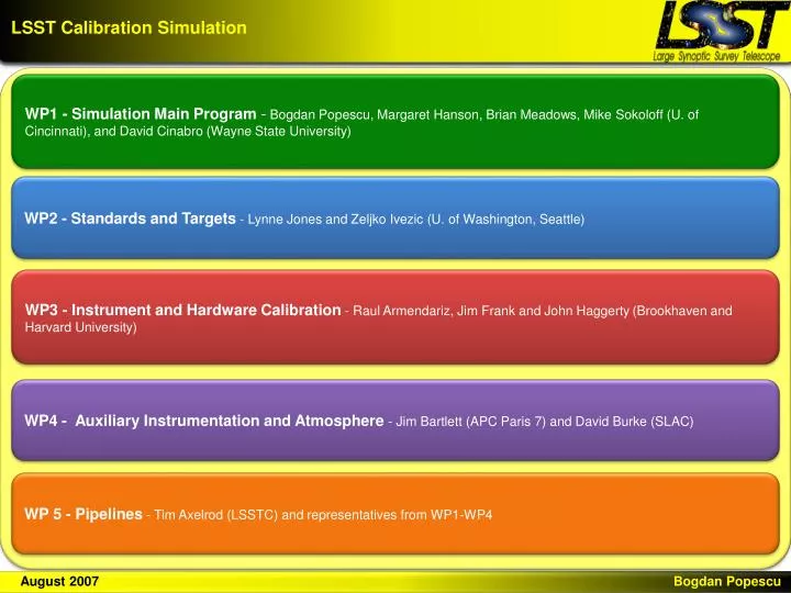
LSST Calibration Simulation. WP1 - Simulation Main Program - Bogdan Popescu, Margaret Hanson, Brian Meadows, Mike Sokoloff (U. of Cincinnati), and David Cinabro (Wayne State University). WP2 - Standards and Targets - Lynne Jones and Zeljko Ivezic (U. of Washington, Seattle).

E N D
LSST Calibration Simulation WP1 - Simulation Main Program - Bogdan Popescu, Margaret Hanson, Brian Meadows, Mike Sokoloff (U. of Cincinnati), and David Cinabro (Wayne State University) WP2 - Standards and Targets - Lynne Jones and ZeljkoIvezic (U. of Washington, Seattle) WP3 - Instrument and Hardware Calibration - Raul Armendariz, Jim Frank and John Haggerty(Brookhaven and Harvard University) WP4 - Auxiliary Instrumentation and Atmosphere - Jim Bartlett (APC Paris 7) and David Burke (SLAC) WP 5 - Pipelines - Tim Axelrod (LSSTC) and representatives from WP1-WP4 August 2007 Bogdan Popescu
LSST Calibration Simulation LSST Calibration Simulation Main Program (WP1) LSST Operations Simulator LSSTFOV(i) Generate References & Standards (WP2) Standard SEDs Simulate Precursor Campaign and Priors (WP2) Standard s Catalog Generate Test Targets (WP2) Target SEDs Generate Instrument Response (WP3) Ir(x,y,n,i) Simulate Calibration Pipeline (WP3) Im(x,y,n,i) Generate Instrument Calibration (WP3) Flats and Bias Generate Aux Telescope Ops (WP4) AUXFOV(j) Simulate Aux Observing(WP4) Aux Object Catalog Zr(az,el,n,i/j) Generate Atmosphere(WP4) Compute Model Source Catalog (WP1) Simulate Image Processing Pipeline (WP5) Model Source Catalog Simulation Analysis and Reporting (WP1) Object Catalog and Zm(az,el,n,i/j) August 2007 Bogdan Popescu
LSST Calibration Simulation - WP1.part1+2 LSST Calibration Simulation Main Program (WP1) i (obsHistID, fieldID), RA and Dec (fieldRA,fieldDec), elevation and azimuth (computed from RA, Dec,etc), camera rotation (rotSkyPos, rotTelPos), filter, date and time (expDate, expMJD, expTime), cloud conditions(xparency), sky brightness (skyBright) LSST Operations Simulator LSSTFOV(i) Generate References & Standards (WP2) Standard SEDs RA and Dec (standard stars), SED's (mean stellar spectra) Simulate Precursor Campaign and Priors (WP2) Standard s Catalog Generate Test Targets (WP2) Target SEDs RA and Dec (targets), SED's (mean stellar spectra) Generate Instrument Response (WP3) Ir(x,y,n,i) ADUs (n,x,y,i) Simulate Calibration Pipeline (WP3) Im(x,y,n,i) Generate Instrument Calibration (WP3) Flats and Bias unknown (at this time) Generate Aux Telescope Ops (WP4) j , RA and Dec , elevation and azimuth(computed from RA, Dec), date and time AUXFOV(j) Simulate Aux Observing(WP4) Aux Object Catalog Zr(az,el,n,i/j) Atmospheric transmission(n) Generate Atmosphere(WP4) Compute Model Source Catalog (WP1)ADUs, i,j, RA and Dec (azimuth, elevation), SEDs Simulate Image Processing Pipeline (WP5) Model Source Catalog Object Catalog and Zm(az,el,n,i/j) Simulation Analysis and Reporting (WP1) August 2007 Bogdan Popescu
LSST Calibration Simulation WP1 - LSSTFOV(i). Elevation, azimuth, camera rotation, filter, date and time, etc from LSST Operations Simulator output file. Indexed sequentially from i=1 to the total number of LSST visits in the observing period. WP2 - Standard and Target SEDs. Top-of-the-atmosphere SEDs for reference (e.g. main sequence), standard (e.g. DA WD) stars, and test science targets (stars, and perhaps galaxies). WP3 - Instrumental Response Ir(x,y,n,i). Response of the telescope and camera to photons (with frequency n) in the telescope pupil from sources on the sky that are imaged with centroid at (x,y) in the focal plane. Output is ADUs in the computer. WP3 - Flats and Biases. Data used in the Calibration Pipeline - dome flats, bias frames, etc. WP4 - AUXFOV(j). Operating parameters for the Auxiliary Telescope (AT); elevation, azimuth, instrument, exposure duration, date and time, etc. Indexed sequentially from j=1 to total number of AT visits in the observing period (not constrained to number of LSST visits). WP4 - Atmospheric Extinction Zr(az,el,n,i/j). Extinction in the atmosphere for both LSST and AUX FOVs. Includes spatial (az,el) and temporal correlations for FOVs i and j. WP1 - Model Image Catalog. Object-indexed catalog of photometric quantities (and others as appropriate) computed from modeled parameters for each LSST visit (two images). Output is in raw ADUs in the computer. August 2007 Bogdan Popescu
LSST Calibration Simulation - UBERCAL UBERCAL - "CMB-like" method (replace CMB temperature fluctuations with the magnitude of stars) Relative calibration achieved using repeated observations. Absolute calibration obtained by comparing with standard stars. That is not a new idea. New : large angular scale and accuracy. The flux : K=K(exposure time, detector efficiency, filter response, telescope optical system, atmosphere, SED) (K gives the absolute calibration) Conversion of flux to magnitude : a(t) = optical response of the telescope and detectors f(i,j;t) = detector flat fields (in magnitudes) (i,j= CCD coordinates) k(t) x = atmospheric extinction (x = airmass = sec(z) in astronomy) ADU - Analog -to-Digital Unit is the digitization of the analog detector output August 2007 Bogdan Popescu
LSST Calibration Simulation - UBERCAL Here t is for one night only; tref = reference time, midnight usually. (a, b, g indexing the appropriate a-term, k-term (and tref) and f-term) j = counts multiple observations; i = ith star. August 2007 Bogdan Popescu
LSST Calibration Simulation - UBERCAL Using a large number of star (table example from SDSS*) and priors for k-terms and flat fields (mean values), the accuracy can be < 1%. Finaly : Relative calibration + Zero Points (for each filter) = Absolute Calibration * Padmanabhan et al, astro-ph/0703454v1 August 2007 Bogdan Popescu
LSST Calibration Simulation - UBERCAL UBERCAL References : Padmanabhan et al, astro-ph/0703454v1 Ivezic et al, astro-ph/0703157v1 August 2007 Bogdan Popescu
Package Description The original plan for creating this package was to allow us to look at the various search methods being applied to find massive clusters in the inner galaxy, and to figure out how these are biased by distance, age, extinction, and compactness of the clusters. We intended to create a simulation of our view of the MW with a variety of assumptions about the distribution of clusters in the MW and to see if current search methods would find any differences. We would base these MW simulations on what is seen in fully face-on galaxies that have a similar star formation rate as the MW. Thus, this would be a reasonable first step towards understanding the distribution and the characteristics of such clusters, since present searches have no way of determining their real 'limit' and sampling biases. August 2007 Bogdan Popescu
Package Description MASSive CLuster - Mcluster = 103 - 104 - 105 - 106 solar masses Evolution - log(Tyears) = 3.00 .. 10.20 ANalysis - HR diagrams, color-magnitude diagrams, FITS images *. MASSCLEAN uses as input a small number of parameters : mass , distance, age, King Model parameters (rt , rc), extinction (AV , RV), metalicity. Using theoretical models - mass distribution (Salpeter IMF), stellar evolution (Geneva Database), spatial distribution (King Model) and extinction (CCM Model) - MASSCLEAN computes actual mass, absolute and apparent magnitude (UBVRIJHK), color indexes, temperature, luminosity and position for all the stars (over 40 000 stars for 105 solar masses cluster) and all the ages included in the Geneva Database. * using SkyMaker (Bertin 2001, Bertin & Fouque 2001-2007) August 2007 Bogdan Popescu
Package Description Mass Geneva Database Mass Distribution Stellar Evolution Salpeter IMF rt , rc Spatial Distribution King Model Cluster Model AV , RV Extinction CCM Model Age August 2007 Bogdan Popescu
RESULTS : Images & Extinction August 2007 Bogdan Popescu
GENEVA DATABASE Advantages : Upper mass limit is 120 solar masses. Fine grid. Age range log(Tyears) = 3.00 .. 10.20 *. UBVRIJHKLM file example : ## ## Isochrone for log(age)= 6.250 # Tracks used: Models with overshooting and OPAL opacities, Z=0.020, 1 X Mdot, Schaller et al. (paper I) # 555 # n M_initM_actlogTefflogglogL M( V) U-B B-V V-R V-I V-K R-I I-K J-H H-K K-L J-K J-L J-L2 K-M # 1 2 3 4 5 6 7 8 9 10 11 12 13 14 15 16 17 18 19 20 21 1 0.8000 0.8000 3.687 4.656 -0.612 6.628 0.847 0.960 0.527 0.949 2.274 0.423 1.319 0.513 0.085 0.076 0.598 0.674 0.676 0.552 2 0.8100 0.8100 3.691 4.654 -0.589 6.549 0.802 0.939 0.515 0.932 2.225 0.417 1.288 0.504 0.083 0.074 0.587 0.661 0.662 0.541 3 0.8200 0.8200 3.695 4.652 -0.566 6.470 0.757 0.917 0.504 0.914 2.175 0.410 1.256 0.494 0.081 0.071 0.575 0.647 0.648 0.530 4 0.8300 0.8300 3.699 4.650 -0.544 6.392 0.711 0.895 0.492 0.896 2.124 0.404 1.224 0.485 0.079 0.069 0.564 0.633 0.634 0.519 .............................................................. # iso_c020_0625. UBVRIJHKLM c = basic grid log(t) range : [3.00,10.20] 0.020 = metalicity Z 0625- log(t)=6.25 August 2007 Bogdan Popescu
RESULTS : Images - Westerlund1 August 2007 Bogdan Popescu
RESULTS : Images - H and CHI PERSEI August 2007 Bogdan Popescu
MASSCLEAN References Alvez, J. et al 2007, A&A,462,L17 Bertin, E. 2001, SkyMaker, http://terapix.iap.fr/cplt/oldSite/soft/skymaker/ Charbonnel, C. et al 1993, A&A, 101, 415 Charbonnel, C. et al 1996, A&A, 115, 339 Charbonnel, C. et al 1999, A&A, 135, 405 Clark, J.S. & Negueruela, I 2002, A&A, 396, L25 Clark, J.S. et al 2005, A&A, 434, 949 Figer,D.F. et al 2006, ApJ, 643, 1166 Gutermuth, R.A. et al 2005, ApJ, 632, 397 Hanson, M. M, Near Infrared tehniques for the study of Massive Star Populations in the Milky Way, in Astronomical Society of the Pacific Conference Series, volume 322, The Formation and Evolution of Massive Young Star Clusters, proceedings of a meeting held in Cancun, Mexico, 2003, 17-21 November Johnstone,D & Bally,J. 2006, ApJ, 653, 383 King, I. 1962, AJ, 67, 471 Lejeune, T. & Schaerer, D. 2001, A&A, 366, 538 Maeder, A. & Meynet, G. 2000, ARA&A, 38, 143 Martins,F. & Plez,B. 2006, A&A, 457, 637 Massey, P. et al 2002, ApJ, 565, 982 Meynet, G. et al 1994, A&AS, 103, 97 Mowlavi, N. et al 1998, A&AS, 128, 471 Muno, M.P. et al. 2006, ApJ, 636, L41 Negueruela, I. & Clark, J.S. 2005, A&A, 436, 541 Oey, M.S. & Clarke,C.J. 2005, ApJ, 620, L43 Piatti, A.E. et al. 1998, A&AS, 127, 423 Salpeter, E.E. 1955, ApJ, 121, 161S Schaerer, D. et al 1993, A&AS, 102, 339 Schaerer, D. et al 1993, A&AS, 98, 523 Schaller, G. et al 1992, A&AS, 96, 269 Westerlund, B. 1961, PASP, 73, 51 August 2007 Bogdan Popescu