Download
1 / 25
280 likes | 641 Vues
Pixel connectivity is a central concept of both edge- and region- based approaches to segmentation. Pixel Connectivity.

E N D
Pixel connectivity is a central concept of both edge- and region- based approaches to segmentation Pixel Connectivity The notation of pixel connectivity describes a relation between two or more pixels. For two pixels to be connected they have to fulfill certain conditions on the pixel brightness and spatial adjacency. First, in order for two pixels to be considered connected, their pixel values must both be from the same set of values V. For a grayscale image, V might be any range of graylevels, e.g.V={22,23,...40}, for a binary image we simple have V={1}. To formulate the adjacency criterion for connectivity, we first introduce the notation of neighborhood. For a pixel p with the coordinates (x,y) the set of pixels given by:
Pixel Connectivity Two pixels p and q, both having values from a set V are 4-connected if q is from the set N4(p) and 8-connected if q is from N8(p) . A pixel p is connected to a pixel q if p is 4-connected to q or if p is 4-connected to a third pixel which itself is connected to q. Or, in other words, two pixels q and p are connected if there is a path from p and q on which each pixel is 4-connected to the next one. A set of pixels in an image which are all connected to each other is called a connected component. Finding all connected components in an image and marking each of them with a distinctive label is called connected component labeling. An example of a binary image with two connected components which are based on 4-connectivity can be seen in Figure 1.
Connected component labeling works on binary or graylevel images and different measures of connectivity are possible.. The connected components labeling operator scans the image by moving along a row until it comes to a point p (where p denotes the pixel to be labeled at any stage in the scanning process) for which V={1}. When this is true, it examines the four neighbors of p which have already been encountered in the scan (i.e. the neighbors (i) to the left of p, (ii) above it, and (iii and iv) the two upper diagonal terms). Based on this information, the labeling of p occurs as follows: Connected Components Labeling • If all four neighbors are 0, assign a new label to p, else • if only one neighbor has V={1}, assign its label to p, else • if one or more of the neighbors have V={1}, assign one of the labels to p and make a note of the equivalences. After completing the scan, the equivalent label pairs are sorted into equivalence classes and a unique label is assigned to each class.
Connected Components Labeling - Examples To illustrate connected components labeling, we start with a simple binary image containing some distinct artificial objects After scanning this image and labeling the distinct pixels classes with a different grayvalue, we obtain the labeled output image Note that this image was scaled, since the initial grayvalues (1 - 8) would all appear black on the screen. However, the pixels initially assigned to the lower classes (1 and 2) are still indiscernible from the background. If we assign a distinct color to each graylevel we obtain One application is to use connected components labeling to count the objects in an image. For example, in the above simple scene the 8 objects yield 8 different classes.
Connected Components Labeling - Examples The full utility of connected components labeling can be realized in an image analysis scenario where images are pre-processed via some segmentation (e.g.thresholding) or classification scheme.
Connected Components Labeling - Examples If we want to count the objects in a real world scene like we first have to threshold the image in order to produce a binary input image (the implementation being used only takes binary images). Setting all values above a value of 150 to zero yields The white dots correspond to the black, dead cells in the original image
Connected Components Labeling - Examples The connected components of this binary image can be seen in The output contains 163 connected components. In order to better see the result, we now would like to assign a color to each component. The problem here is that we cannot find 163 colors where each of them is different enough from all others to be distinguished by the human eye.
Connected Components Labeling - Examples Two possible ways to assign the colors are as follows: 1) We only use a few colors (e.g.8) which are clearly different from each other and assign each graylevel of the connected component image to one of these colors. The result can be seen in • We can now easily distinguish two different components, provided that they were not assign the same color. However, we lose a lot of information because the (in this case) 163 gray levels are reduced to 8 different colors. 2) We can assign a different color to each gray value, many of them being quite similar. A typical result for the above image would be • Although, we sometimes cannot tell the border between two components when they are very close to each other, we do not lose any information
Connected Components Labeling - Examples If we compare the above color-labeled images with the original, we can see that the number of components is quite close to the number of dead cells in the image. However, we obtain a small difference since some cells merge together into one component or dead cells are suppressed by the threshold.
Connected Components Labeling - Examples We encounter greater problems when trying to count the number of turkeys in this image Labeling the thresholded image yields Although we managed to assign one connected component to each turkey, the number of components (196) does not correspond to the number of turkeys.
Connected Components Labeling - Examples The two last examples showed that the connected component labeling is the easy part of the automated analysis process, whereas the major task is to obtain a good binary image which separates the objects from the background.
Labeling data output from a classification processes We can classify multi-spectral images (e.g. a two-band image consisting of (visible range) and (infra-red range)) in order to find k groupings of the data based on the pixel intensities clusters
Labeling data output from a classification processes The multi-spectral image was classified into two groups. If we now apply connected components labeling, connected geographic regions which belong to the same intensity classes can be labeled. The result contains 49 different components, most of them being only a few pixels large. One could now use this image to further investigate the regions, e.g. if some components changed their size compared to a reference image or if other regions merged together.
Edge detection algorithms typically are followed by linking procedures to assemble edge pixels into meaningful edges One of the simplest approach for linking edge points is to analyze the characteristics of pixels in a small neighborhood ( 3 x 3 , 5 x 5) We can compare 1) the strength of the response of the gradient operator used to produce the edge pixel and 2) the direction of the gradient vector. This comparison can be made as follows for a pixel (x,y) and pixel(x’,y’) in its neighborhood . . Pixel (x,y) has similar magnitude to pixel ( x’,y’) if Edge Linking and Boundary Detection Pixel (x,y) has an angle similar to pixel (x’y’) A point in the predefined neighborhood of (x,y) is linked to the pixel at ( x,y) if both magnitude and direction criteria are satisfied.
Region –Based Segmentation The uniformity or otherwise of a connected region of pixels may be indicated by a uniformity predicate. A logical statement that is true only if pixels in the region are sufficiently similar in terms of gray level, color or some other property. where (j,k) and (m,n) are the coordinates of neighboring pixels in region R. where f(j,k) is the grey level of a pixel from region R with coordinates (j,k) and r is a mean grey level of all pixels in R except the pixel at (j,k)
Region Oriented Segmentation • Let R represent the entire image region, and let P(Ri) represent a logical predicate over the points in set Ri. Then, we may view segmentation as a process that partitions R into n subregions, R1, R2, ...., Rn , such that
Region Oriented Segmentation • Condition(1) indicates that; • The segmentation must be complete, that is, every pixel must be in a region. • Condition(2) indicates that; • The points in a region must be connected. • Condition(3) indicates that; • The region must be disjoint. • Condition(4) indicates; • The properties that must be satisfied by the pixels in a segmented region. • Condition(5) indicates that; • The regions Ri and Rj are different in the sense of predicate P.
Region Growing • Region growing is a bottom-up procedure that starts with a set of seed pixels. The aim is to grow a uniform connected region from each seed. A pixel is added to a region if and only if : • - It has not been assigned to any other region. • It is a neighbor of that region. • The new region created by addition of the pixel is still uniform. http://marathon.csee.usf.edu/range/seg-comp/SegComp.html http://www.caip.rutgers.edu/~comanici/segm_images.html
Limitations of region growing Note that a complete segmentation of an image must satisfy a number of criteria: 1)All pixels must be assigned to regions 2)Each pixel must belong to a single region only 3)Each region must be a connected set of pixels 4)Each region must be uniform 5)Any merged pair of adjacent regions must be non-uniform Region growing satisfies the third and fourth of these criteria, but not the others. It fails to satisfy the first and second criteria because, in general, the number of seeds defined by the user will not be sufficient to create a region for every pixel. The fifth criterion is not satisfied because the regions grown from two nearby seeds are always regarded as distinct, even if those seeds are defined in a part of the image that should be segmented as a singe region.
The Split and Merge Algorithm • A complete segmentation is possible if we adopt a top-down approach, in which the entire image is considered initially to be a single region. If P(image) is FALSE, we divide the image into four quadrants. If P is FALSE for any quadrant, we subdivide that quadrant into sub quadrants and so on . • Split into four disjoint regions Ri for which P(Ri) .= FALSE • Merge any adjacent regions Rj and Rk for which P(Rj Rk) = TRUE • Stop when no further merging or splitting is possible.
Segmentation - Conclusions • identify pixels that belong to features of interest • first step in automatic image analysis and interpretation • applications involving detection, recognition, or measurement of features • non-contextual techniques • - ignore relationships between pixels of a feature • - group pixels based on a global attribute • contextual • - exploit relationships between pixels of a feature (e.g. proximity)
* non-contextual approach *used for solid objects resting on a contrasting background * may threshold on gray level * generates a binary image - assign 1 (or 255) to pixels with gray levels of interest - assign 0 to the rest * may have one or two thresholds * may implement via a lookup table * picking the threshold is the hard part --human operator - GrayMapTool application --preselected threshold --mean gray level --fixed percentage of pixels selected --choose a point between two peaks in the histogram Thresholding - Conclusions
Contextual techniques for image segmentation • pixels belonging to the same object are close to each other • we look at proximity as well as gray level • approaches based on discontinuity • e.g. use edge detection to identify the boundary of a region • can be difficult to generate a complete boundary (no holes) • approaches based on similarity • - group pixels together based on similarity and proximity • - specify similarity criteria
Contextual techniques for image segmentation - Conclusions pixel connectivity region labeling after thresholding region similarity region growing split and merge Examples: http://trident.mcs.kent.edu/~nochiai/ThesisD/thesis_menu.html http://viper.unige.ch/research/segmentation/index.html