Download
1 / 21
250 likes | 583 Vues
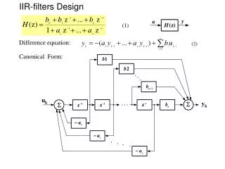
(1). Difference equation:. IIR-filters Design. (2). Canonical Form:. u k. y k. Im. R=1. z 1. Re. Restrictions:. (1). General form:. (2). Amplitude response:. |W(z)| 2 =W(z)W(z -1 ). Phase response:. (3). (4). (5). (6). (7). Design of Analog Prototypes. General form:. (8).

E N D
(1) Difference equation: IIR-filters Design (2) Canonical Form: uk yk
Im R=1 z1 Re Restrictions: (1) General form: (2) Amplitude response: |W(z)|2 =W(z)W(z-1). Phase response: (3) (4) (5) (6) (7)
Design of Analog Prototypes General form: (8) General form for Butterworth, Chebyshev, Bessel, Caurer (elliptic) filters: (9) Butterworth LP- filter: (10) (11) (12) (12) After Wiener factorization of (11):
(13) (14) Normalized transfer function: (15) Non-normalized transfer function: (16) For case (14,15): (17) For case (16):
Zero-pole Map of Butterworth Filter (18)
[n, Wn]=buttord(0.25,0.4,1,60) N=14, Wn=0.2658 [b,a]=butter(n,Wn); fvtool(b,a) For analog prototype: [n, Wn]=buttord(0.25,0.4,1,60,’s’) Converting analog prototype to digital filter: - Bilinear transform (19) (20) [numd,dend]= bilinear(num,den,fs); or: [numd,dend]= bilinear(num,den,fs,fp); - Invariance of impulse response (21) (22) (24)
[bz,az]=impinvar(b,a,fs); [bz,az]=impinvar(b,a,fs,tol)); Design of Butterworth Filter in MATLAB %Butterworth filter design Fs=1000; %sampling frequence tm=0:1/Fs:0.5;%time vector %Data vector: k=2;am=3; z=am*cos(2*pi*50*tm); x=z+k*randn(size(tm)); %low-pass filter design specification objectives: d=fdesign.lowpass('N,F3db',5,100,Fs); %order=5, edge frequency=100 %Invoke Butterworth filter design method Hd=design(d,'butter'); y=filter(Hd,x); %results of filtering figure(1); subplot(2,1,1),plot(tm,x,'b'), grid on subplot(2,1,2),plot(tm,y,'k',tm,z,'m'), grid on %design results visualization fvtool(Hd)
x z y Results of Filtering Maxflat filters n = 10; % order of polynomial in denominator m= 2; % order of polynomial in numerator Wn = 0.25; % normalized cutoff frequency [b,a]=maxflat(n,m,Wn); fvtool(b,a)
Bessel Filters (1) Bessel Functions (2) Cut off frequency: (3) n=5; %order Wn=1000; [b,a]= besself(5,1000) % Wn – edge frequency of band, within which
Chebyshev Filters (4) Chebyshev polynomials: (5) Amplitude of ripples in the pass band: (6) [b,a] = cheby1(n,Rp,Wn,options) n=4; Rp=1 (dB); Ω=0.4 Roots of denominator are located on the ellipse:
Chebyshev 1 Chebyshev 2 [b,a]=cheby2(n,R,Wst,’ftype’) n=4, R=30, Wst=0.4. [A,B,C,D]=cheby2(n,R,Wst,’ftype’) [z,p,k]=cheby2(n,R,Wst,’ftype’)
Elliptic filter [b,a] = ellip(n,Rp,Rs,Wn,options) [z,p,k] = ellip(n,Rp,Rs,Wn,options) [A,B,C,D] = ellip(n,Rp,Rs,Wn,options) n=6, Rp=1, Rs=40, Wn=0.25
Conversion of filters Basic filter in MATLAB is lp-filter with normalized edge frequency Wn=1 rad/sec 2) [bt,at] = lp2hp(b,a,Wo) [At,Bt,Ct,Dt] = lp2hp(A,B,C,D,Wo) 1) [bt,at] = lp2lp(b,a,Wo) [At,Bt,Ct,Dt] = lp2lp(A,B,C,D,Wo) 3) [bt,at] = lp2bs(b,a,Wo,Bw) [At,Bt,Ct,Dt] = lp2bs(A,B,C,D,Wo,Bw) 4) [bt,at] = lp2bp(b,a,Wo,Bw) [At,Bt,Ct,Dt] = lp2bp(A,B,C,D,Wo,Bw) Example (case 2):
Integrating IIR-filters 1. Rectangular formula: (1) (2) (3)
2. Trapezoid formula: (4) (5) (6)
3. Simpson’s formula: (7) (8) (9)
Fast Convolution Based on FFT (10) (11) (12)
Block-diagram of the Fast Convolution with Overlapping and Storage Algorithm H(n) y(n) x(k) Output control& storage FFT IFFT Frames & Overlap Y(n)=H(n)X(n) x(k) Alg. Ov & St L L h(k) 2N-1 3N-1 kT N-1 L L N N 1st frame y(n) n N N 2nd frame 3rd frame
ADAPTATION TO THE VARIATIONS OF THE PLANT’S MAGNITUDE FREQUENCY RESPONSE