Download
1 / 37
370 likes | 461 Vues
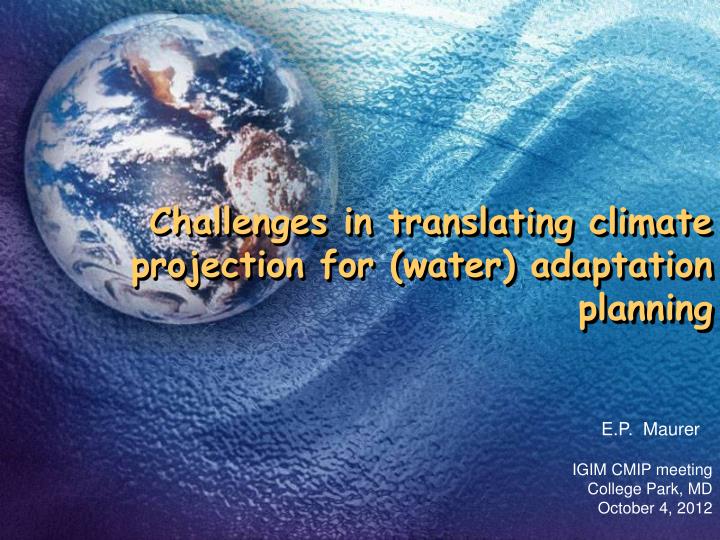
Challenges in translating climate projection for (water) adaptation planning. E.P. Maurer. IGIM CMIP meeting College Park, MD October 4, 2012. A well-meaning hydrologist walks into a climate change study…. Estimating Climate Impacts to Water. 2. Global Climate Model.

E N D
Challenges in translating climate projection for (water) adaptation planning E.P. Maurer IGIM CMIP meeting College Park, MD October 4, 2012
A well-meaning hydrologist walks into a climate change study…
Estimating Climate Impacts to Water 2. Global Climate Model 4. Land surface (Hydrology) Model 1. GHG Emissions Scenario 5. Operations/impacts Models • “Downscaling” Adapted from Cayan and Knowles, SCRIPPS/USGS, 2003
Selecting GCM runs: “Bookends” Brackets range of uncertainty Useful where impacts models are complex Downscale output from few GCMs
Bookend results for California • CA average annual temperatures for 330-year periods • Amount of warming depends on our GHG emissions at end of 21st century. • Summer temperatures increases (end of 21st century) vary widely: • Lower: 3.5-6 °F • Higher: 6-10.5 °F Ref: Luers et al., 2006, CEC-500-2006-077 and Cayan et al., 2006, CEC-500-2005-203-SF
Downscaling: bringing global signals to regional scale GCM scale and processes at too coarse a scale Figure: Wilks, 1995 • Resolved by: • Bias Correction • Spatial Downscaling
BCSD Method – “BC” • At each grid cell for “training” period, develop monthly CDFs of P, T for • GCM • Observations (aggregated to GCM scale) • Obs are from Maurer et al. [2002] • Use quantile mapping to ensure monthly statistics (at GCM scale) match obs • Apply same quantile mapping to “projected” period Wood et al., BAMS 2006
Raw GCM Output Precip, Temp Downscaling for Hydrology Impact Modeling • BCSD downscaling of GCM Precip and Temp • Use to drive VIC model • Obtain runoff, streamflow, snow
Projected Impacts: Loss of Snow • Snow water in reserve on April 1 • Change (Sacramento-San Joaquin basin, 2 GCMs, 2 emissions scenarios): -12% to -42% (for 2035–2064) (up to 1 Lake Shasta) -32% to -79% (for 2070–2099) (up to 2 Lake Shastas) Ref: Luers et al., 2006, CEC-500-2006-077 GFDL CM2.1 results
Some Agency and Organizational Responses Background: Confederation Bridge in the Gulf of Saint Lawrence (http://www.cakex.org)
IPCC CMIP3 GCM Simulations • 20th century through 2100 and beyond • >20 GCMs • Multiple Future Emissions Scenarios http://www-pcmdi.llnl.gov/
Multi-Model Ensemble Projections for Feather River • Increase Dec-Feb Flows • 77% for A2 • 55% for B1 • Decrease May-Jul • 30% for A2 • 21% for B1
2/3 chance that loss will be at least 40% by mid century, 70% by end of century Point at: 120ºW, 38ºN Impact Probabilities for Planning Snow water equivalent on April 1, mm • Combine many future scenarios, models, since we don’t know which path we’ll follow (22 futures here) • Choose appropriate level of risk
Monthly downscaled data • PCMDI CMIP3 archive of global projections • 16 GCMs, 3 Emissions • 112 GCM runs • Allows quick analysis of multi-model ensembles • gdo4.ucllnl.org/downscaled_cmip3_projections
Use of U.S. Data Archive • Thousands of users downloaded >20 TB of data • Uses for Research (R), Management & Planning (MP), Education (E)
A1B Scenario Source: Girvetz et al, PloS, 2009 Global BCSD • Similar to US archive, but ½-degree • Publicly available since 2009 • Captures variability among GCMs • www.engr.scu.edu/~emaurer/global_data/ • Data accessed by users in all 50 States and 99 countries (last 11 months only)
Online Analysis and Download withhttp://ClimateWizard.org Level 1 Level 2 Level 3 • Global and US data sets • Country and US state boundaries defined • Spatial and time series analysis • Upload of custom shapefiles Girvetz et al., PLoS, 2009
Too much information? • Little guidance in selection of: • Emissions • GCMs • Hundreds of downscaled GCM runs • Many impacts studies cannot use all of them • How much information is really useful?
Selecting Specific GCM Runs • Bivariate probability plot shows correlation between T, P • Identify Change Range: 10 to 90 %-tile T, P • Select bounds based on: • risk attitude • interest in breadth of changes • number of simulations desired Brekke et al., 2009
Selecting GCMs for Impact Studies • Ensemble mean provides better skill • Little advantage to weighting GCMs according to skill • Most important to have “ensembles of runs with enough realizations to reduce the effects of natural internal climate variability” [Pierce et al., 2009] • Maybe 10-14 GCMs is enough? Gleckler, Taylor, and Doutriaux, Journal of Geophysical Research (2008) as adapted by B. Santer Brekke et al., 2008
Do CMIP GCM runs capture important uncertainties? • Perturbed physics ensembles • Is planning for the higher probability outcomes appropriate? Roe and Baker, 2007
Downscaling for Extreme Events • Some impacts due to changes at short time scales • Heat waves • Flood events • Daily GCM output limited for CMIP3, more plentiful for CMIP5 • Downscaling adapted for modeling extremes
Library of previously observed anomaly patterns: Coarse resolution analogue: P2 P1 p2 p1 Constructed Analogues Given daily GCM anomaly Analogue is linear combination of best 30 observed Apply analogue to fine-resolution climatology
Sustainable Design in a Dynamic Environment • Declining return periods for extreme events • A solution: Overdesign for present Das et al, 2012 Mailhot and Sophie Duchesne, JWRPM, 2010
What is missing from downscaled data original archive? Downscaled data run through VIC model, now available
Archive expansion (still CMIP3) • Daily downscaled data • Hydrology model output
Is bias correction effective? Biases vary in time, space, at quantiles • On average, bias correction works • But for small ensembles maybe not
CMIP5 additions to archive • Monthly downscaling of Tmax, Tmin, Precip for: • 84 historical GCM runs • 237 projections (total for 4 RCPs) • Daily downscaling with two techniques: • 46 historical runs • 147 projections (total for 4 RCPs) • Hydrology model output for 100 runs
Does CMIP3 or CMIP5 choice matter? • Ensemble average changes comparable • RCP8.5 and SRES A2 comparable
Model Spread • Differences in model spread between CMIP3 and CMIP5 varies by location
Information overload overload • If 112 GCM projections wasn’t too much, is 500? • Have we progressed in providing policymakers with information for… • Selecting concentration pathways • Assembling an ensemble of GCMs • Using appropriate downscaling • Interpreting results • Can we (conditionally) recommend anything?