Download
1 / 12
120 likes | 386 Vues
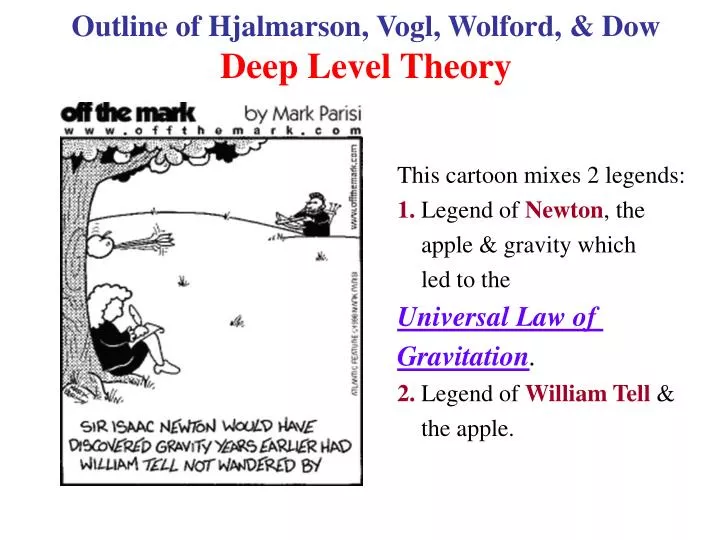
Outline of Hjalmarson, Vogl, Wolford, & Dow Deep Level Theory. This cartoon mixes 2 legends: 1. Legend of Newton , the apple & gravity which led to the Universal Law of Gravitation . 2. Legend of William Tell & the apple.

E N D
Outline of Hjalmarson, Vogl, Wolford, & Dow Deep Level Theory This cartoon mixes 2 legends: 1. Legend of Newton, the apple & gravity which led to the Universal Law of Gravitation. 2. Legend of William Tell & the apple.
A brief outline of this theory, then some results. • The Schrödinger Equation including the defect or impurity is (Dirac notation, for convenience): (Ho +V)|Ψ> = E|Ψ> (1) Ho=Hamiltonian for a perfect, periodic, crystal. It produces the bandstructure. V =The defect potential (to be discussed). It produces defect levels. • Solve (1) in r space (the direct lattice) to take advantage of the localized nature of Vfor deep levels. Use a tightbinding (LCAO) approach to the bandstructure & a Green’s function formalism. See YC, Ch. 4, which discusses this in detail. • Manipulate with (1) (using an operator or matrix formalism): (E- Ho)|Ψ> = V|Ψ> or|Ψ> = (E- Ho )-1 V|Ψ> or[1 - (E- Ho )-1V]|Ψ> = 0 Finally det[1 - (E- Ho )-1V] = 0 (2) Emphasize:(2) the Schrödinger Equation(1) in different notation!
So, the Schrödinger Equation including the defect or impurity is det[1 - (E- Ho )-1V] = 0 (2) • It is convenient to define the Host Green’s Function(Matrix)Operator Go(E) (E- Ho)-1 • The Schrödinger Equation(2) then has the form: det[1 - Go(E)V] = 0 (3) The GOAL is then: Given Ho, & V, find the energy E which makes the determinant in (3) vanish! (3) is an equation for the deep level E, which is the eigenvalue of the Hamiltonian with the defect, H = Ho+ V & the solution to the Schrödinger Equation we seek!
det[1 - Go(E)V] = 0 (3) • To solve (3), models for Ho (bandstructures) & V (defect potential) are needed. • The calculations use a tightbinding (LCAO) representation for Ho & V, and for the Green’s function Go(E). • For the host bandstructures Ho use the formalism in the paper: “A Semi-Empirical Tightbinding Theory of the Electronic Structure of Semiconductors” P. Vogl, H. Hjalmarson, & J. Dow, Journal of the Physics and Chemistry of Solids, 44, 365-378 (1983) (directly linked from the course lecture page). • For the defect potential V, use the formalism in the paper: “Theory of Substitutional Deep Traps in Covalent Semiconductors”, H. Hjalmarson, P. Vogl, D. Wolford, & J. Dow Physical Review Letters44, 810 (1980). (directly linked from the course lecture page). See also, H.P. Hjalmarson, PhD dissertation, U. of Ill., 1980
det[1 - Go(E)V] = 0 (3) Hjalmarson Deep Level Theory: • Rather than a quantitative theory, it is a theory designed for & best suited for predictions of chemical trends in deep levels (discussed next) & explanations of such trends. • It & generalizations have been successfully used to predict chemical trendsin a variety of problems. Its simplicity allows for qualitative & semi-quantitative predictions of a number of defect properties. It’s quantitative accuracy is limited. Chemical Trends • Given the host, how does the deep level change as the impurity is changed or as one type of defect is changed to another. • Given the impurity or defect, how does the deep level change as the host changes(especially, the alloy composition dependence in alloy semiconductors). • Explaining chemical trends will help to explain a lot of data!
det[1 - Go(E)V] = 0 • Consider substitutional impurities only at first. • The host Hois described by Vogl, Hjalmarson, Dow semi-empirical tightbinding bandstructures. • Model for theDefect Potential V: • Considers the central cell part ofVonly. Neglects the long ranged Coulomb potential. There are no shallow(hydrogenic)levels in this theory (these could be accounted for later using EMT!) • Considersidealdefects only, neglects lattice relaxation. (Generalized to include this by W.G. Li & C.W. Myles in the late 1980’s) • Considers nearest-neighbor interactions only. • V is a diagonal matrix in the LCAO representation. • Considers neutral impurities only: No charge state effects (added later by Lee & Dow).
det[1 - Go(E)V] = 0 • Model for the Defect Potential V.Assume that: • V is diagonal & proportional a difference in “atomic energies” between impurity & host atom it replaces. • The matrixV = H - Ho. In the LCAO representation, the diagonal matrix elements are “atomic energies, so the diagonal elements of V have the form: Vℓ (εI)ℓ- (εH)ℓ Here (εI)ℓ& (εH)ℓare the impurity & the host atomic energies for the orbital of symmetry type ℓ(ℓ = s, p, d,…) or (ℓ = A1, T2, ….) That is Vℓ βℓ[(εI)ℓ- (εH)ℓ] βℓis an empirical parameter. • This form explicitly accounts for chemical shifts & their effects on the defect potential.
So, finally: det[1 - Go(E)V] = 0(1) • Vis a diagonal matrix with diagonal elements Vℓ = βℓ[(εI)ℓ- (εH)ℓ](2) • Given V, the Ewhich solves (1) is the deep level of interest. • Independently of (2), for given Vgiven, (1) can be viewed as An IMPLICIT EQUATION (with a numerical solution) for the deep levelE as a function of V. • That is, (1) can be thought of as a function: E = E(V) (3) • Now, using (2), (3) becomes E = E(εI)(4) • Numerical solution to (4) gives predictions ofChemical Trends!
From this graph, we obtain the implicit function E = E(εI) That is, it predicts how the deep level E depends on the impurity. Or, it predicts a chemical trend! det[1 - Go(E)V] = 0 (1) Vℓ = βℓ[(εI)ℓ- (εH)ℓ] (2) • A plot of the numerical results forEvs. the diagonal part of Vor, equivalently Eversus (εI)ℓlooks schematically like: • For a specific impurity (fixed V or fixed atomic energies), drop a vertical line from that V. Where this crosses the curve (the solution to (1)), is the predicted deep level. A1(s-like) levels are shown. Other symmetries are similar. E specific impurity Vℓ or(εI)ℓ
Consider N in GaP & GaAs • An Example of a “Good” Deep Center • The short-ranged potential means that the wavefunction in r space will be highly localized around the N. • The electron wavefunction is spread out in k-space. • Although GaP is an indirect bandgap material, the optical • transition is very strong in GaP:N • Red LED’s used to be made from GaP:N • It turns out that a large amount of N can be introduced • into GaP but only small amount of N can be introduced • into GaAs because of a larger difference in atomic sizes. 14
N in GaP • A “Good” Deep Center • The N impurity in GaP is a “good” deep center because it makes GaP:N into a material which is useful for light-emitting diodes (LED). • GaPhas an indirect band gap so, pure GaP is not a good • material for LED’s(just as Si & Ge also aren’t for the same reason). • It turns out that the presence of N actually enhances the • optical transition from the conduction band to the N level which makes GaP:Nan efficient emitter. • So, GaP:N was one of the earliest materials for red LED’s. • More recently, GaP:Nhas been replaced by the more efficient emitter: GaInP (alloy). 13
The GaAsP Alloy with N Impurities:Interesting, beautiful data! • The N impurity level is a • deep level in the bandgap • in GaP but is a level • resonant in the conduction • band in GaAs. The figure • is photoluminescence data • in the alloy GaAsxP1-x:N • under large hydrostatic • pressure for various alloy • compositions x. 13