Download
1 / 42
420 likes | 547 Vues
CMAQ Multi-Pollutant Response Surface Modeling: Applications of an Innovative Policy Support Tool. CMAS Conference – October 17, 2006 Session 2: Analysis Methods and Tools USEPA/OAQPS - Sharon Phillips, Bryan Hubbell, Carey Jang, Pat Dolwick, Norm Possiel, Tyler Fox. Outline.

E N D
CMAQ Multi-Pollutant Response Surface Modeling: Applications of an Innovative Policy Support Tool CMAS Conference – October 17, 2006 Session 2: Analysis Methods and Tools USEPA/OAQPS - Sharon Phillips, Bryan Hubbell, Carey Jang, Pat Dolwick, Norm Possiel, Tyler Fox
Outline • Overview of Response Surface Model (RSM) • Need for the RSM • Define RSM • Development of multi-pollutant RSM using CMAQ • Steps in designing CMAQ RSM applications • Experimental design • CMAQ – SMOKE interface development • Evaluation & Validation • RSM outputs / Visual Policy Analyzer • CMAQ RSM application results • Next steps
Need for Response Surface Model • Growing importance of AQ models in guiding and supporting policy analysis and implementation for complex AQ issues such as PM, O3, and air toxics • Enormous computational costs (time & resources) always present a challenge for time pressing need of policy analysis • Current model operation in comparing the efficacy of various control strategies and policy scenarios is typically inefficient, if not ineffective • An innovative policy support tool to address these issues in an economical manner is needed
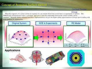
What is a Response Surface Model? • Response Surface Model (RSM) is a “reduced form” model of a complex air quality model (e.g. CMAQ) – “meta-model” • Based on a systematically selected set of model runs, statistical techniques can be used to represent the relationship between model inputs and outputs (e.g. emissions control and concentrations of PM & ozone) • Once the “response surface” has been generated, it can be used to simulate the functions of the more computationally expensive photochemical air quality model • Cross-validation can then be conducted to examine the validity of RSM to represent model responses • Can also be used to derive analytical representations of model sensitivities to changes in model inputs
How the RSM can be used • Strategy design and assessment screening tool • Comparison of urban vs. regional controls • Comparison across sectors • Comparison across pollutants • Optimization • Can be used to develop optimal combinations of controls to attain standards at minimum cost • “What If?” Analyses • provide real-time predictions of model responses to model inputs • Quickly provide insights into questions for policy design, e.g. does is it matter whether regional controls are put in place before local controls? • Model sensitivity • Can be used to systematically evaluate the relative sensitivity of modeled ozone and PM levels to changes in emissions/met inputs
Elements in the Development of a RSM • Policy objectives • Model requirements • Geographic scale • Output metrics • Experimental design • Selection of policy factors • Specification of air quality model simulations • Air quality modeling simulations • Statistical analysis and development of predictive model • Visualization software tool
Development Plan for Response Surface Model Determine Relevant Policy Factors Assess Policy Objectives Determine Output Metrics Develop Experimental Design Select Base Inventory Run Modeling Experiments Process Model Outputs Model Validation for PM Response Metrics Build Predictive Model Develop Emissions Summaries Develop Response Surface Summary Metrics Development of Visual Policy Analysis Tool Evaluate Relative Effectiveness of Policy Factors
RSM Pilot Applications: History RSM for PM2.5 using REMSAD RSM for O3 using CAMx (Strategy Comparison) NOx controls VOC controls VOC controls vs. NOx controls
Development of CMAQ RSM Applications • Determine policy objectives • Experimental design • Selection of policy factors • Emission control factors • Regional vs. urban control • Selection of air quality model simulations • Continental U.S. modeling, 2010 CAIR Base, 36-km grid resolution • 210 runs (in 3 stages) for 4 months (Feb., April, July, Dec.) • CMAQ – SMOKE Interface Development • Develop a module within CMAQ to read directly the pre-merged SMOKE sector files (e.g., 3-D point, 2-D mobile, etc.) • Allow RSM to directly control % changes of (1) emissions and (2) specified areas • Output Metrics • Response Surface Variables • Validation and Evaluation • Cross-validation • Out-of-sample validation
Policy Objectives • Provide a modeling surrogate tool that can quickly simulate the PM and ozone impacts for a variety of control strategies for use in Regulatory Impact Analyses (e.g., PM NAAQS, O3 NAAQS) • For screening level estimates of the impacts of control strategies on NAAQS design values • For use in generating screening estimates of the health benefits of reductions in PM and ozone precursors • Provide air quality simulation tool for use in the Air Strategy Assessment Program (ASAP), a screening tool under development that evaluates the relative air quality impacts, costs, and health benefits of controlling emissions from different sources
Experimental Design: (1) Selection of control factors • 12 emission control factors selected based on precursor emissions & source category relevant to policy analysis of interest
Factors Provide Reasonable Aggregation Omitted • Source groupings with smaller contributions to emissions are grouped with similar larger source groupings for efficiency • NonEGU Area NOx and SO2 sources are primarily smaller industrial combustions sources such as coal, oil, and natural gas powered boilers and internal combustion engines • Agricultural area sources are only significant contributors to ammonia emissions • VOC sources are lumped together because VOCs are not expected to influence PM levels significantly Combined Combined Combined Omitted
Experimental Design: (1) Selection of control factors • Covers from zero to 120 percent of baseline emissions • Staged Latin Hypercube (space filling design) • 210 total runs, 120 runs in first stage, 60 runs in stage two and 30 boundary condition runs • Will allow testing of additional predictive power of additional model runs • 30 additional model validation runs
Experimental Design: (1) Selection of control factors • Regional vs. Urban control:independent response surfaces for9 urban areas, as well as a generalized response surface for the rest of model domain • Nine urban areas include: NY/Philadelphia, Chicago, Atlanta, Dallas, San Joaquin, Salt Lake City, Phoenix, Seattle, and Denver • Selected so that ambient PM2.5 in each urban area is largely independent of the precursor emissions in all other included urban areas
CMAQ – SMOKE Interface: Timely & Efficient Development of Model-ready Emissions Region A (9 urban areas) Region B (rest of domain)
Experimental Design: (2) Selection of Model Simulations • CMAQ model simulations • CMAQ v4.4; 14 vertical layers • Domain = Continental U.S. 36-km CAIR modeling domain • 4 months, one from each season, February, April, July, October (months selected to provide best prediction of quarterly mean) • Baseline Emissions Data • CAIR 2010 Base Case • Includes Tier 2, Heavy Duty Diesel Engines, and Nonroad Diesel standards, as well as the NOx SIP Call and MACT standards CMAQ Modeling Domain
Output Metrics (Response Variables) • Quarterly mean and annual 98th percentile daily average: sulfate, nitrate, crustal, elemental carbon, organic carbon, ammonium • PM2.5 annual and daily design values (at monitored locations) • Annual/Seasonal nitrogen and sulfate deposition • Visibility (light extinction): annual mean, average of 20% worst days, average of 20% best days • Ozone summer averages for: • 8hr max, 1hr max, 5hr avg, 8hr avg, 12hr avg, 24hr avg • Ozone 8-Hour design values (at monitored locations)
RSM Validation and Evaluation • Cross-validation • for each RSM iteration, one of the model runs was left out, the RSM is computed and used to predict the omitted run • RSM predicted changes in AQ are compared with CMAQ predictions and the mean square error (MSE) over all grid cells was computed for the run • Out-of-sample validation • 30 additional CMAQ runs were conducted (not part of the experimental design and were not used in developing RSM) • RSM predictions for these model runs were compared with the CMAQ predictions and the MSE over all grid cells was computed for each run
Cross-Validation: Comparison of RSM Predicted to CMAQ “true” Values forJuly PM2.5 mass ** based on an evenly geographically distributed sub-sample of 700 grid cells, out of ~6,300 in the continental U.S. July total PM2.5 mass (sample of 700 grid cells)
Cross-Validation: Comparison of RSM Predicted to CMAQ “true” Values forOctober PM2.5 mass ** based on an evenly geographically distributed sub-sample of 700 grid cells, out of ~6,300 in the continental U.S. October total PM2.5 mass (sample of 700 grid cells)
Similarity of Geographic Patterns of Predicted PM2.5 (mean total) changes for October based on Run 120 RSM CMAQ
RSM Graphical Tool: Visual Policy Analyzer • Graphical analysis tool to allow for “real-time” RSM predictions of ozone, PM, visibility, and deposition • Continuous improvements are implemented to the user interface and functions
2-Way Response Surfaces for Chicago NR VOC NR NOx Onroad VOC Onroad NOx
Quick re-cap • RSM can analyze air quality changes in 9 urban areas and associated counties independently of one another • For each urban area: • Input to RSM: • % local or regional reduction for one or more of the 12 factors • Output from RSM: • Estimated changes in air quality at peak monitor in each county on an annual and daily basis • Gridded air quality changes across urban area • To estimate regional emission reductions reduces the regional emission reduction % in the entire rest of US, which is outside of the 9 urban areas
VPA example: Monitors with annual average PM2.5 Post CAIR 2015 greater than 13 µg/m3
VPA example: Monitors with annual average PM2.5 Post CAIR 2015 greater than 13 µg/m3 after applying 50 percent reduction in carbon
Example of Air Quality Impacts: “Regionality” of SO2 vs. “Locality” of Carbon SO2 Carbon
Key Local Factors are Carbon, EGU SO2, NonEGU SO2, VOC, and NH3 Key Regional Factors are EGU SO2, NonEGU SO2, Area NH3, and Carbon Availability of controls may limit the ability to achieve the desired percent reductions in specific sources and pollutants that would result in reductions in ambient PM2.5 levels to meet the attainment targets.
Relative effectiveness per ton in reducing ambient PM2.5 levels is only one factor in determining the appropriateness of controls. Cost effectiveness per microgram is the more complete measure, and reflects both the atmospheric response and costs of the controls.
What types of reductions have the biggest local effect on PM2.5 in the East?
Next Steps • Planning for 12km “Local Scale” RSM for selected areas of concern (FY06/FY07) • Implementation of multi-pollutant ASAP version using CMAQ RSM • Use RSM results to investigate/guide sector based O3/PM analyses • Collaboration & outreach to AQ community (RPOs, academic, international, etc.) to facilitate transfer of methods and development of RSM tools
Development of CMAQ Response Surface Model Determine Relevant Policy Factors Universe of Potential Factors Factor Elimination Process Assess Policy Objectives Time/Resources Tradeoff Matrix CMAQ/CAMx Limits Determine Output Metrics (Response Variables) Select Air Quality Model Emissions Inventories Develop Experimental Design(Battelle) Preliminary Modeling Select Base Inventory (projection year + base control set) Specify Modeling Domain (including nested subgrids) Select Model Grid Size (e.g. 12km or 36 km) Run Modeling Experiments Specify Modeling Periods (e.g. 4 months, one from each season) Develop Emissions Summaries (Annual or Daily Emissions by Factor) Evaluation of 2001 full year CMAQ results Process Model Outputs (compute response variables) PM2.5 and Ozone Monitoring Data Model Validation for Ozone and PM2.5 Response Metrics Build Predictive Model FLOWCHART KEY Develop Normalized Adjustment Ratios (SMAT technique for PM2.5, BenMAP eVNA for Ozone) PREPARATION Develop Response Surface Summary Metrics Development of Visualization Tool (Batelle) And Integration into ASAP DATA/INPUT PROCESS Evaluate Relative Effectiveness of Policy Factors Evaluate Relative Cost-Effectiveness And Calculate optimal factor levels DECISION
PM2.5: Areas of Influence for All 9 Urban Locations July 2001 (monthly avg.) February 2001 (monthly avg.)
Areas of Influence for Selected Urban Locations New York/Philadelphia Chicago PM2.5 July monthly avg. Atlanta Small overlaps between Chicago and NY influences in Ohio and Western NY. No overlap between Atlanta and NY Small overlaps between Atlanta and Chicago influences in Western KY
Extent of Air Quality Influence Region for 9 Selected Urban Areas
CMAQ Application: Analyzing Illustrative Control Scenarios • Analyze sequence of controls • Demonstrates ways in which states might meet the standard • Each bin contains multiple control options • Iterate analysis to identify mix of local and regional controls • Use RSM to help optimize for cost and monetized human health benefits Baseline Modeling (e.g CAIR) (1) Local Controls Initial Iteratation Subsequent Iteration (2) Non-EGU Regional Controls (3) Local-Scale Targeted EGU Controls as Proposed by States
Relative Impacts of 30 Percent Reductions in Precursor Emissions Across Source Categories Included in the Response Surface Model Chicago 2015 Annual Design Value = 16.9
Relative Impacts of 30 Percent Reductions in Precursor Emissions Across Source Categories Included in the Response Surface Model San Joaquin 2015 Annual Design Value = 21.7
2-Way Response Surfaces for NY NR VOC NR NOx Onroad VOC Onroad NOx