Download
1 / 72
730 likes | 851 Vues
H331: Computer Graphics. http://www.cs.kuleuven.ac.be/~graphics/H331/ Philip Dutré Department of Computer Science Wednesday, March 19. Today. Ray Tracing (Chapter 14). http://www.oyonale.com/ressources/english/mkofwetbird1.htm. How did we generate pictures so far?. Viewing transform

E N D
H331: Computer Graphics http://www.cs.kuleuven.ac.be/~graphics/H331/Philip Dutré Department of Computer Science Wednesday, March 19
Today • Ray Tracing(Chapter 14) http://www.oyonale.com/ressources/english/mkofwetbird1.htm
How did we generate pictures so far? • Viewing transform • camera in origin • Perspective transform • Clipping • Scan-conversion • Z-buffer for visibility
Ray tracing • RT is a more powerful technique to render scenes • For each pixel: • What surface point is visible through this pixel? (“trace a ray …”) • What color does this point have? • No perspective transform, no clipping, …
Basic RT algorithm: set-up • Camera defined by eyepoint and view plane in world space screen environment eyepoint
Basic RT algorithm: viewing rays • Send a ray from the eye through each pixel • Intersect ray with all geometry in the scene screen environment eyepoint
Basic RT algorithm: viewing rays • If a ray hits an object, that object is shown • … otherwise, background color is shown screen environment eyepoint
Viewing rays screenv yres pixels (0..yres-1) ray origin = eye ray direction = d - screenh - screenv + (xres+.5)*screenh/||screenh|| + (yres+.5)*screenv/||screenv|| d screenh eye xres pixels (0..xres-1)
Basic RT algorithm • Evaluate shading model for each point, e.g.:
RT: skeleton • For each pixel (x,y): • Construct the ray for pixel (x,y) • Intersect the ray with all objects in the scene • Pick the closest intersection, in front of the eye • Compute the color of the hitpoint, w.r.t. lightsources • Color pixel
Ray-Sphere intersection • Sphere is centered at c, radius = R • Surface intersection point p defined twice: • (px-cx)2 + (py-cy)2 + (pz-cz)2 = R2 (equation for sphere) • e + t.dir = p (equation of ray) • Combining equations: • (ex-cx+t.dirx)2 + (ey-cy +t.diry)2 + (ez-cz +t.dirz)2 = R2 • Solving quadratic for t yields 0, 1, 2 intersections
Ray-Transformed object intersection • Apply inverse transform to ray • Intersect transformed ray with original object • Apply transform to intersection point
Ray-Transformed object intersection • Transform ray only once transform all objects • Exact location of hitpoint & normal need to be transformed back!
Ray – CSG Intersections: Easy!!! • Find intersections with operand objects • Apply operand to intersection spans Objects Union Intersection Difference
Ray / Object intersection questions • Closest hit: t>= 0, or t>= epsilon ? • Backface culling? • Normal vector at hit point: • Needed for shading • Transformed objects? • Local parametrization (u,v)for intersection point • Needed for texture mapping, bump-mapping etc.
Texture mapping v y t u surface x s pixel on screen texture map
Bump mapping (u,v) used to perturbate normal shading looks different
Bump mapping Color Plate from “Advanced Animation and Rendering Technique” by Alan Watt and Mark Watt
RT and shadows • Trace shadow-ray to light source • If shadow-ray hits something shadow screen environment eyepoint
RT and shadows • Trace shadow-ray to light source • If shadow-ray hits something shadow screen environment eyepoint
RT and shadows No shadow test Shadow-ray intersection test
RT and shadows • Shadow Ray: • Origin = point to be shaded • Direction: towards the (point) light source • Actual intersection point not important • If we find ANY point between point to be shaded and light source shadow • We do not have to find the closest one • Can be made slightly more effective
Reflections and transparancy • So far: • Direct illumination (shading model) • Shadows • One viewing ray for each pixel • Indirect light? • Reflections: light coming from perfect specular direction • Refractions: light coming from perfect refractive direction
Reflections and transparancy • Shoot perfect reflected ray, find closest hitpoint • Add color of this hitpoint to current hitpoint screen environment eyepoint
Reflections and transparancy • Reflected ray: • Origin: hitpoint • Direction: perfect reflected direction • Shading model: Recursive ray tracing
Reflections and transparancy • Shoot perfect refracted ray, find closest hitpoint • Add color of this hitpoint to current hitpoint screen environment eyepoint
Reflections and transparancy • Refracted ray: • Origin: hitpoint • Direction: perfect refracted direction (Snell’s law) • Shading model:
Very first raytraced picture (Whitted 1980)
Comparisons (Cornell PCG)
Recursive Ray Tracing T 2 N Surface normal R i N 2 R T 2 3 1 R Reflected ray i N 3 R L Shadow ray 1 i T Transmitted ray L 3 i L L 2 1 N 1 Point light source Viewpoint
Recursive Ray Tracing: how to stop? • Fixed depth • When contribution to original pixel falls below threshold • Successive reflections/refractions diminish contribution of ray • Adaptive tree pruning
Is ray tracing slow or fast? • Traditional ray tracing is O(N*P) • N objects • P pixels • One shadow ray for each light source • Recursive rays • … many, many rays!!!
Making RT Faster • Faster ray-object intersections • Bounding volumes • Fewer ray-object intersections • Bounding volumes hierarchies • Spatial subdivision techniques
Bounding Volumes • Put a simple enclosure (BV) around an object • Test ray against BV • If hit, then test ray against object • If miss, we know object is missed
Bounding Volumes • BV should be simple to test • BV should be tight
Bounding Volumes • Cost per ray = intersect_cost_BV + intersect_cost_object * prob_ray_hits_BV Keep this cheap Keep this small (very tight) (simple BV)
Bounding Volumes • Can be organised in hierarchy
Bounding Volumes • Most popular • Spheres • Axis-aligned cuboids • Projection extents • 2D rectangular bounding volume around projection of object on screen (p. 788)
Space Subdivision • Basic idea: • Divide space into cells • Store relevant objects in each cell • Trace ray from cell to cell, only intersect with objects in current cell
Space subdivision • Efficient for all rays • Uses a lot of memory • Bad for irregular spaced models in the scene (many empty cells) • Overhead: trace ray from cell-to-cell