Download
1 / 23
230 likes | 665 Vues
Version 1/9/2001. FINANCIAL ENGINEERING: DERIVATIVES AND RISK MANAGEMENT (J. Wiley, 2001) K. Cuthbertson and D. Nitzsche Lecture Value at Risk: Mapping . Topics .

E N D
Version 1/9/2001 FINANCIAL ENGINEERING: DERIVATIVES AND RISK MANAGEMENT(J. Wiley, 2001) K. Cuthbertson and D. Nitzsche Lecture Value at Risk: Mapping Copyright K.Cuthbertson, D. Nitzsche
Topics VaR for Different Assets (Mapping) StocksForeign AssetsCoupon Paying BondsOther Assets(All of above have portfolio returns that are approximately ‘linear’ in individual returns ~ hence use VCV method) Copyright K.Cuthbertson, D. Nitzsche
Your Cash : Is it Safe in Their Hands ? • * Copyright K.Cuthbertson, D. Nitzsche
VaR for Different Assets (Mapping) Copyright K.Cuthbertson, D. Nitzsche
VaR for Different Assets: Practical Issues • PROBLEMS • STOCKS : Too many covariances [= n(n-1)/2 ] • FOREIGN ASSETS : Need VaR in “home currency” • BONDS: Many different coupons paid at different times • DERIVATIVES: Options payoffs can be highly non- linear (ie. NOT normally distributed) Copyright K.Cuthbertson, D. Nitzsche
VaR for Different Assets: Practical Issues • SOLUTIONS = “Mapping” • STOCKS : Within each country use “single index model” SIM • FOREIGN ASSETS : Treat asset in foreign country = “local currency risk”+ spot FX risk • BONDS: treat each bond as a series of “zeros” • OTHER ASSETS: Forward-FX, FRA’s Swaps: decompose into ‘constituent parts’. • DERIVATIVES: ~ next lecture Copyright K.Cuthbertson, D. Nitzsche
Stocks/Equities and SIM Copyright K.Cuthbertson, D. Nitzsche
“Mapping” Equities using SIM • Problem : Too many covariances to estimate • Soln. All n(n-1)/2 covariances “collapse or mapped” into m and the asset betas (n-of them) • Single Index Model: • Ri = ai + bi Rm + ei • Rk = ak + bk Rm + ek • assume Ei k = 0 and cov (Rm , e) = 0 • All the systematic variation in Ri AND Rk is due to Rm ‘p’ = portfolio of stocks held in one country (Rm , m) for eg. S&P500 in US Copyright K.Cuthbertson, D. Nitzsche
Intuition 1) In a diversified portfolio s2 (i ) =0 2) Then each return-i depends only on the market return (and beta). Hence ALL variances and covariances also only depend on these 2 factors. We then only require( n-betas + s2m )to calculate ALL our inputs for VaR. 3) = 1 because (in a well diversified portfolio) each return moves only with Rm 4) We end up with [1]VaRp = Vpbp (1.65sm ) or equivalently VaRp = (Z C Z’ )1/2 where C is the unit matrix Copyright K.Cuthbertson, D. Nitzsche
THE MATHS OF SIM AND VaR - OPTIONAL ! SIM implies: i,k =cov(Ri,Rk )= bibk s2m i,2 = var(Ri) = b2is2m + s2 (i ) BUT in diversified portfolio s2 (i ) = 0 and = 1 Copyright K.Cuthbertson, D. Nitzsche
THE MATHS OF SIM AND VaR - OPTIONAL ! • We have(linear): Rp = w1R1 + w2 R2 + …. • From the SIM we can deduce that for a PORTFOLIO of equities in one country • Standard Deviation of the PORTFOLIO is given by : sp = bp sm where: bp = Swi bi • (ie. portfolio beta requires, only n-beta’s) • Hence: [1]VaRp = Vpbp (1.65sm ) Copyright K.Cuthbertson, D. Nitzsche
Alternative Representation • Eqn [1] above can be written: • VaRp = (Z C Z’ )1/2 • where: • VaR1 = V1 1.65 ( b1m ) and VaR2 =V2 1.65 ( b2m) • Z = [ VaR1 , VaR2 ] • C is the identity matrix C = ( 1 1 ; 1 1 ), since = 1 for the SIM and a well diversified portfolio. Copyright K.Cuthbertson, D. Nitzsche
SIM: Checking the Formulae • [1] VaRp = Vpbp (1.65sm ) = Vp ( Swi bi) (1.65sm) • = (V1 b1 + V2 b2 ) (1.65sm) • The above can easily be shown to be the same as • VaRp = (Z C Z’ )1/2 • = (1.65 m) [ (V1 b1)2 + (V2 b2)2 + 2 V1 b1 V2b2 ]1/2 • where VaR1= V1 1.65( b1m) • VaR2 =V2 1.65 ( b2 m ) • and Z = [ VaR1 , VaR2 ] and C = ( 1 1 ; 1 1 ) Copyright K.Cuthbertson, D. Nitzsche
“Mapping” Foreign Assets into Domestic Currency Copyright K.Cuthbertson, D. Nitzsche
“Mapping” Foreign Assets into Domestic Currency • US based investor with DM140m in DAX • Two sources of risk • a) variance of the DAX • b) variance of $-DM exchange rate • c) one covariance/correlation coefficient • (between FX-rate and DAX) • eg. Suppose when DAX falls then the DM also falls - ‘double whammy’ from this positive correlation Copyright K.Cuthbertson, D. Nitzsche
“Mapping” Foreign Assets into Domestic Currency • US based investor with DM140m in DAX • FX rate : S = 0.714 $/DM ( 1.4 DM/$ ) • Dollar initial value Vo$ = 140/1.4 = $100m • Linear R$ = RDAX + R$/DM • above implies wi = Vi / V0$ = 1 and • p = • Dollar-VaRp = Vo$ 1.65 p • r = correlation between return on DAX and FX rate Copyright K.Cuthbertson, D. Nitzsche
“Mapping” Foreign Assets into Domestic Currency Alternative Representation Dollar VaR Let Z = [ V0,$ 1.65 sDAX , V0,$ 1.65 sS ] = [ VaR1 , VaR2 ] V0,$ = $100m for both entries in the Z-vector Then VaRp = (Z C Z’ )1/2 Copyright K.Cuthbertson, D. Nitzsche
“Mapping”Coupon Paying Bonds Copyright K.Cuthbertson, D. Nitzsche
“Mapping”Coupon Paying Bonds • Coupons paid at t=5 and t=7 • Treat each coupon as a separate zero coupon bond • P is linear in the ‘price’ of the zeros, V5 and V7 • We require two variances of “prices” V5 and V7 and • covariance between these prices. • 5(dV / V) = D (dy5) Copyright K.Cuthbertson, D. Nitzsche
Coupon Paying Bonds • Treat each coupon as a zero • Calculate PV of coupon = price of zero, V5 = 100 / (1+y5)5 • VaR5 = V5 (1.65 s5) • VaR7 = V7 (1.65 s7) • VaR (both coupon payments) • = • r = correlation: bond prices at t=5 and t=7 • (approx 0.95 - 0.99 ) Copyright K.Cuthbertson, D. Nitzsche
Mapping on to “standard” RMetrics Vertices $ 100 m Actual Cash Flow 5 6 7 RM Cash Flow 5 7 Weights , 1- , are chosen to ensure weighted average volatility based on RM values of at 5 and 7 equals the interpolated volatility at “6” Copyright K.Cuthbertson, D. Nitzsche
“MAPPING” OTHER ASSETS • SWAP: • = LONG FIXED RATE BOND AND SHORT AN FRN • FRA (6m x 12m) • = BORROW AT 6 MONTHS SPOT RATE +LEND AT 12M SPOT RATE • FORWARD FX: • = BORROW AND LEND IN DOMESTIC AND FOREIGN SPOT INTEREST RATES AND CONVERT PROCEEDS AT CURRENT SPOT-FX Copyright K.Cuthbertson, D. Nitzsche
End of Slides Copyright K.Cuthbertson, D. Nitzsche