Download
1 / 21
210 likes | 957 Vues
Approaches to the measurement of excess risk. 1. Ratio of RISKS 2. Difference in RISKS: (risk in Exposed)-(risk in Non-Exposed). Risk in Exposed Risk in Non-Exposed. Measures of RISK in Epidemiologic Studies. Without an explicit Comparison Absolute risk With an explicit comparison

E N D
Approaches to the measurement of excess risk • 1. Ratio of RISKS • 2. Difference in RISKS: • (risk in Exposed)-(risk in Non-Exposed) Risk in Exposed Risk in Non-Exposed
Measures of RISK in Epidemiologic Studies • Without an explicit Comparison • Absolute risk • With an explicit comparison • Relative risk • Odds ratio • Attributable risk
Cohort Study …then follow to see whether: a a+c c c+d = Incidence in exposed a a+b c c+d Relative Risk = = Incidence in Non-exposed
Hypothetical cohort study of the 1-year incidence of Acute Myocardial Infarction in indivduals with Severe Hpertension (180 mm Hg) and Normal Systolic blood Pressure (<120 mm Hg) 180 9820 30 9970 0.018 0.003 0.01833 0.00301 = = 6.09 Adapted from M. Szkly & J Nieto; Epidemiology: beyond the basics.
When is the Odds Ratio a Good Estimate of the Relative Risk? • When the “cases” studied are representative of all people with the disease in the population from which the cases were drawn, with regard to history of the exposure; • When the “controls” studied are representative of all people without the disease in the population from which the cases were drawn, with regard to history of exposure; • When the disease being studied is not a frequent one.
Incidence of Local Reactions in the Vaccinated and Placebo Groups, Influenza Vaccination trial Note: Based on data for individuals 40 years old or older in Seltser et al. To avoid rounding ambiguities in these and subsequent examples based on these data, the original sample sizes in Seltser et al.’s study (257 vaccinees and 241 placebo recipients) were multiplied by 10. Source: Data from R Seltser, PE Sartwell, and JA Bell, A Controlled test of Asian Influenza Vaccine in Population of Families, Am J. of Hygiene, 1962 (75):112-135. Adapted from M. Szkly & J Nieto; Epidemiology: beyond the basics.
Cross-tabulation of exposure and disease in a cohort study a b c d c c+d c c+d q- c d = = 1-q- 1 -
An expression of of the mathematical relationship between the OR on the one hand and the relative risk on the other, can be derived as follows. Assume that q+ is the incidence (probability) in exposed (e.g. vaccinated) and q- the incidence in unexposed individuals. The odds ratio is then: q+ 1-q+ q- 1-q- q+ 1-q+ 1-q- q- q+ q- 1-q- 1-q+ = x OR = = x 1-q- 1-q+ Notice that the term q+/q- in the equation is the relative risk. Thus the term defines the bias responsible for the discrepancy between the relative risk and odds ratio estimates (built-in bias). If the association between the exposure and the outcome is positive, q- < q+, thus (1-q-) > (1-q+). The bias term will therefor be greater than 1.0, leading to an overestimation of the relative risk by the odds ratio. By analogy, if the factor is protective, the opposite occurs - that is, (1-q-) < (1-q+) - and the odds ratio will again overestimate the strength of the association. In general, the odds ratio tends to yield an estimate further away from 1.0 than the relative risk on both sides of the scale (above or below 1.0).
Do the math: 1. Using the hypertension/myocardial infarct example RR= OR= OR=RR x “built in bias = 2. Using the example of local reactions to the influenza vaccine RR= OR= OR=RR x “built in bias =
Cohort studyA sample of exposed and non-exposed Incidence among smokers = 84/3000=28.0 Incidence among non-smokers = 87/5000=17.4
Attributable Risk The incidence in smokers which is attributable to their smoking - Incidence in smokers Incidence in Non-Smokers The ARexp of CHD attributable to smoking is:
Percent ARexp • A percent ARexp (%ARexp) is simply the ARexp expressed as a percentage of the risk in the exposed (q+). The excess risk associated with the exposure as a percentage of the total q+. • For a binary exposure, it is • %ARexp = q+ - q- x 100 • q+ • The %ARexp in the CHD/Smoking example is:
Population Attributable Risk • PAR is dependent on the population prevalence of exposure. • As the population is composed of exposed and unexposed individuals, the incidence in the population is similar to the incidence in the unexposed when the exposure is rare (A). • Incidence in the population is closer to that in the exposed, when the exposure is common (B).
Population Attributable Risk (PAR) and its dependence on the population prevalence of the exposure A. Pop ARexp ARexp Pop ARexp B. ARexp
Incidence in the total population, which is due to the exposure, can be calculated by subtracting: [Incidence in the total population] – [Incidence in the non-exposed group] In order to calculate this, one must know: EITHER: the incidence in the total population, OR: the incidence among smokers, the incidence among non-smokers, AND: the proportion of the total population with the exposure, i.e., the proportion of the population that smokes in the population under study or from which incidence can be calculated
We KNOW: incidence among smokers = 28.0/1,000/year, And, the incidence among non-smokers = 17.4/1,000/year. If we assume that from some other source of information, we know that the proportion of smokers in the population is 44% (and therefor the proportion of non-smokers is 56%), then the incidence in the total population can be calculated as: [28.0/1,000] [.44] + [17.4/1,000] [.56] = 22.0/1,000 SO THAT: [Incidence in the total population] – [Incidence in the non-exposed group] = [22.0/1,000/year] – [17.4/1,000/year] – 4.6/1,000/year
And the proportion of the incidence in the total population, which is attributable to the exposure, can be calculated by: • [Incidence in the total population] – [Incidence in the non-exposed group]-- • Incidence in the total population • = 22.0 – 17.4 = 20.9% • 22.0 • i.e., there should be a total reduction of 20.9% in the incidence of CHD in this population if smoking were eliminated.
Levin’s formula for the attributable risk for the Total Population After simple arithmetic manipulation, the previous formula can be expressed as a function of the prevalence of the exposure in the population and the relative risk : p (RR-1) x 100 p (RR-1) + 1 where p = proportion of the population with the characteristic or exposure and RR= relative risk or Odds Ratio (if applicable)
PAR: dependence on prevalence of exposure and relative risk RR=10 RR=5 RR=3 RR=2 For all values of the relative risk, the population AR increased markedly as the exposure prevalence increases.