Download
1 / 54
550 likes | 764 Vues
Empirical approaches to trade modeling- cge and partial equilbrium Lecture 12: aheed course “international agricultural trade and policy” Taught by alex f. mccalla , professor emeritus, uc-davis April 6, 2010 university of tirana , albania. Lecture drawn from IFPRI materials.

E N D
Empirical approaches to trade modeling-cge and partial equilbriumLecture 12: aheed course “international agricultural trade and policy”Taught by alex f. mccalla, professor emeritus, uc-davisApril 6, 2010 university of tirana, albania Lecture drawn from IFPRI materials
Approaches to Trade Modeling • There are basically three widely used techniques of modeling trade: • Computable General Equilibrium Models (CGEs); • Partial Equilibrium Models (PEMs) frequently of two sub-types; • Spatial equilibrium models which model physical distances; • Non-spatial models which link countries with transport cost functions (PEM-NS) • Econometric Models such as Gravity Trade Flow Models.
2 IFPRI Models • We will look at two types of models used most frequently in trade analysis-CGEs and PEM-NS: • The first ids the IFPRI IMPACT Model, a PEM-NS, where I will share slides provided by SiwaMsangi of IFPRI; • The second is the IFPRI MIRAGE CGE model. I will share slides provided byAntoineBouet of IFPRI. • Thanks to both of them and IFPRI
The IMPACT Model and Planned Improvements in the Global Futures Project Global Futures Launch Meeting 1 March 2010, IFPRI, Washington, D.C. Siwa Msangi + team…
Overview • Introduction to the IMPACT Model • Coverage (spatial, commodity) • Basic equations (“the guts”) • Linkages to well-being outcomes (esp. nutrition) • Key data (what goes in) + outputs (what comes out) • Typical applications – what it does and does not do • Key linkages with exogenous ‘drivers’ of change given by biophysical models – in particular, climate change • Global Futures enhancements • Conclusions
The IMPACT Model • IMPACT – “International Model for Policy Analysis of Agricultural Commodities and Trade” • Representation of a global competitive agricultural market for crops and livestock • Global • 115 countries • 281 food production units • 32 agricultural commodities
32 IMPACT Commodities • Cereals • Wheat, Rice, Maize, Other Coarse Grains + Millet, Sorghum • Roots & Tubers • Potatoes, Sweet Potatoes & Yams, Cassava & Other Roots and Tubers • Dryland legumes • Chickpea, Pigeonpea, Groundnut • Livestock products • Beef, Pork, Sheep & Goat, Poultry, Eggs, Milk • Fish • Eight capture and aquaculture fish commodities plus fish meals and fish oils • High-Value • Vegetables, (Sub)-Tropical Fruits, Temperate Fruits, Sugar Cane, Sugar Beets and Sweeteners • Other • Soybeans, Meals, Oils • Non-food • Cotton, Biofuel products (ethanol, biodiesel)
Global Food Production Units (281 FPUs) Higher river basin spatial resolution planned for better water availability modeling
IMPACT Basics • Global, partial-equilibrium, multi-commodity agricultural sector model • Links country-level supply and demand through global market interaction and prices • Country-level markets are linked to the rest of the world through trade • World food prices are determined annually at levels that clear international commodity markets
Policy drivers Domestic Biofuel Prodn Other Demand Demand Socioeconomic Drivers Feed Food Agric. Imports/ exports Trade Equilibrium Balance Trade policy child malnutrition Price Calorie Availability Irrigation investments Area Female education Clean water access Supply Rural Roads Yield [investments] Ag R&D investments Climate change Environmental driver Key linkages in modeling drivers & outcomes Page 12
IMPACT Equations: Production QS = quantity produced A = crop area, irrigated and rainfed Y = crop yield, irrigated and rainfed t = time index n = country/FPU index i = commodity indices specific for crops
IMPACT Area and Yield Functions • Area – function of crop prices and other sources of growth (exogenous and others modeled) • Yield – function of crop and input price, and other sources of growth • Underlying yield growth are implicit policy drivers that are not directly embedded in the simulation • Public and private research • Markets, infrastructure, irrigation investments
IMPACT Equations: Area Response, at FPU Level A = crop area α = crop area intercept PS = effective producer price ε = area price elasticity WAT = water stress = exogenous area growth rate (can be altered to reflect urbanization, climate change, etc.
IMPACT Equations: Yield Response, at FPU Level Y = crop yield β = crop yield intercept PS = effective producer price g= yield price elasticity k = inputs such as labor and capital PF = price of factor or input k = exogenous yield growth rate WAT = water stress
IMPACT Food Demand, at Country Level • Food demand is a function of commodity prices, income, and population • Income (gI) and population (gP) growth rates exogenous Use CGE modeling to endogenize
IMPACT Feed Demand • Feed demand is a function of livestock production, feed prices, and feeding efficiency • l = commodity indices specific for livestock commodities • b = commodity indices specific for feed commodities
IMPACT Other Demand • Other demand grows in the same proportion as food and feed demand • In the case of biofuel – this other category represents the feedstock demand for particular commodities
IMPACT Total Demand • Total demand is the sum of food, feed, and other demand
IMPACT Price Determination • Prices are endogenous • Domestic prices – function of world prices, adjusted by effect of price policies, expressed as producer subsidy equivalents (PSE), consumer subsidy equivalents (CSE), and the marketing margin (MI). • MI currently single value per country. Will make spatial Producer Prices Consumer Prices Feed Prices
IMPACT Net Trade • Commodity trade is the difference between domestic production and demand. Countries with • positive trade are net exporters • negative values are net importers For some commodities, stock change would be included in this equation – the methodology is currently under revision
IMPACT Market Clearing Condition • Minimize the sum of net trade with a world market price for each commodity that satisfies the market-clearing condition
Number and Percentage Malnourished Children Malnourished children are projected as follows: %ΔMALt= - 25.24 * Δt-1 ln (PCKCAL) - 71.76 Δt-1 LFEXPRAT - 0.22 Δt-1SCH - 0.08 Δt-1 WATER NMALt = %MALt x POP5t %MAL = Percent of malnourished children PCKCAL = Per capita calorie consumption SCH = Total female enrollment in secondary education as a % of the female age-group LFEXPRAT = Ratio of female to male life exp. at birth WATER = Percent of people with access to clean water NMAL = Number of malnourished children, and POP5 = Number of children 0 to 5 years old
IMPACT Starting Values • 2000 FAOSTAT. Will update to 2005 • ISPAM 5 minute production and area data (also tuned to 2000 FAOSTAT). Will update to 2005 • HarvestChoice product • Plausible allocation of 20 crops (soon to be 30) spatially based on agroclimatic conditions and known regional production statistics • Hydrology uses Univ. of East Anglia data, and streamflow is calibrated to WaterGAP model results • Prices based on World Bank ‘pink sheets’ and other sources • Elasticity values taken from previous IMPACT values, and adjusted for the purposes of calibration in some cases
IMPACT Outputs • Supply • Demand (food, feed, and other demand) • Net trade • World prices • Per capita demand • Number and percent of malnourished children • Calorie consumption per capita • Plus • Water use, (at some point: soil carbon, total biomass)
The Bread & Butter of IMPACT • Much of the past work of IMPACT has centered around providing a forward-looking perspective on what’s needed to meet future food needs, and the implications for key CGIAR mandate commodities • Because it was designed to look at the long term, that aren’t covered by others (USDA, FAPRI, OECD), the results are better used for projections and not prediction – which implies that you’re more interested in deviations from a baseline, under alternative scenarios, rather than point estimates • Can be useful for determining which crop improvements have the biggest effect on food availability and levels of malnutrition
Typical IMPACT-driven scenarios • Looking at the implications of socio-economic growth (income, population) on food/feed demand and other indicators mentioned above • Looking at the implications of higher factor prices (fertilizer, labor) on crop yield – and production • Fairly simple trade liberalization or protection scenarios (with phased changes over time) • Looking at implications of improved socio-economic conditions ( access to clean water, girls secondary schooling, rural roads ) on child malnutrition
Issues that IMPACT cannot cover • Explicit projections on poverty or household-level income changes • Modeling the endogenous feedbacks between input prices and agricultural output and price changes • Going directly from agricultural gross production value (revenue) to total agricultural value-added • Going from changes in implied changes in child malnutrition levels to changes in number of total malnourished in the population (except by assumption, perhaps….) • Other implications for non-agricultural sectors…
Applications of IMPACT • The IMPACT model is used most often for long run projections but also can be used for trade policy analysis. • Chapter 4 in McCalla & Nash by Mark Rosegrant & Siet Meijer presents the results of four trade liberalization scenarios: • In terms of impacts on cereal and livestock trade; • Impacts on commodity prices; • Economic benefits of trade liberalization.
Training sessions on the MIRAGE model and on the MAcMap-HS6 database The MIRAGE model – Structure and Theory Antoine Bouet David Laborde Marcelle Thomas Rabat, Mars 2010
Presentation of the MIRAGE model • Data sources = inputs for the model • Main hypotheses of the model
Presentation of the MIRAGE model MIRAGE = Modeling International Relationships in Applied General Equilibrium Brief reminder: • CGEM devoted to trade policies analysis • Multi-country • Multi-sector • 5 primary factors • Perfect & Imperfect competition • Horizontal (variety) & Vertical (quality) differentiation • Static vs. Dynamic (sequential)
Data sources • The calibration of the MIRAGE model is computed from data for a base year • 2 main data sources: • GTAP v. 6.1 database (2001) or GTAP v. 7 database (2004) • MAcMap-HS6 database (2004)
Data sources GTAP = Global Trade Analysis Project • Purdue University (USA, Indiana) • Data on world trade (bilateral flows,…), production, consumption, intermediate use of commodities and services • Disaggregation (GTAP 7) covering (57 sectors and 113 regions) • New regions added to version 7 include: Armenia, Azerbaijan, Belarus, Bolivia, Cambodia, Costa Rica, Ecuador, Egypt, Ethiopia, Georgia, Guatemala, Iran, Kazakhstan, Kyrgyzstan, Laos, Mauritius, Myanmar, Nicaragua, Nigeria, Norway, Pakistan, Panama, Paraguay, Senegal and Ukraine ( https://www.gtap.agecon.purdue.edu/ ) • Interest: use this Global database as a Global Social Accounting Matrix for the MIRAGE model
Data sources MAcMap-HS6 = Market Access Maps • ITC (UNCTAD-WTO) and CEPII • Data on market access (bilateral applied tariff duties - taking into account regional agreements and trade preferences; information given at the HS6 level) • Data come from: national sources and IDB (Integrated DataBase) from the WTO (http://www.ifpri.org/book-5078/ourwork/program/macmap-hs6) • Interest: replace tariffs coming from GTAP database by the ones coming from MAcMap-HS6 into the MIRAGE model
Presentation of the MIRAGE model Main hypotheses of the model
General Structure • MIRAGE = Modeling International Relationships in Applied General Equilibrium • r,sregions • i,jGoods • Input/Output tables and bilateraltrade • I*R*S and I*J*R: large number of flows • One representative agent per region • Five factors • Firms per sector: • One in perfectcompetition • N homogenous in imperfectcompetition
Main hypotheses of the model • Production factors • Skilled labor: perfect mobility between sectors • Unskilled labor: imperfect mobility between agricultural and non agricultural sectors - perfect mobility amongst each group’s sectors ; another specification is possible: Lewis model in some Dvg countries • Land: imperfectly mobile between sectors • Natural resources: sector-specific and constant • Capital: sector-specific and accumulative
Demand Three types of demand: final consumption: LES-CES function intermediate consumption: CES capital good (from fixed saving rate on revenues): CES Supplied by domestic production or imports Several levels of differentiation: Quality (2 geographical zones) Domestic vs. imports if in same quality zone Differentiation by regions within each quality zone
Main hypotheses of the model Final Consumption: LES-CES function Linear Expenditure System - Constant Elasticity of Substitution • The demand structure of each region depends on its income level (i.e.: a minimum level of the final consumption is assumed for each region according to the income level of which one the consumer is issued) • In MIRAGE, minimum levels of consumption: • 1/3 for developed countries • 2/3 for developing countries • All others characteristics as a CES function • New version of the MIRAGE model: new calibration procedure of the CES – LES in order to generate price and income elasticities which are compatible (by sectors and regions) with those estimated by USDA-ERS.
Main hypotheses of the model • Product differentiation (3 levels by nested Armington) Armington hypothesis: choice between products based on geographical origins (differentiations by geographical origins) • 2nd level : 2 quality ranges from geographical basis → 2 zones • Zone U = regions from the same quality of the region of the buyer • Zone V = regions from the other quality In MIRAGE, goods produced by developed countries are assumed to have a different quality than the ones produced by developing countries)
Main hypotheses of the model • 3rd level: same hypothesis inside a same Zone of quality (vertical differentiation: local goods are assumed to be different than foreign ones • Local region • Foreign regions • 4th level: same hypothesis inside foreign regions: goods produced inside each foreign region are assumed to be different than the one produced each other one • Foreign region 1 • … • Foreign region n • … • Foreign region N
Main hypotheses of the model • Product differentiation: horizontal differentiation (in case of imperfect competition only) • 5th level: Dixit-Stiglitz differentiation which implied a difference in variety among the goods • Characteristics: same as a CES function with 1 innovation → Allow the number of arguments to be variable
Main hypotheses of the model • Imperfect competition characteristics • Cournot-Nash oligopolistic competition • Number of firms = number of varieties • Increasing returns to scale modeled by a fixed cost in terms of output (calibrated for profits=0 in the base year) • In the short term, positive mark-up depending on demand elasticity • In the long term adjustment of the number of firms such that profits go down to 0 • Number of firms/varieties, substitution elasticities and markups calibrated jointly in order to minimize an objective given estimated values that are not fully consistent with each other
Specifications of factor markets • Segmentation of unskilled labour market • Developed countries • CET: Segmentation between urban sectors and rural sectors • Developing countries • Can be changed considering unrestricted labour reserve in rural areas of high populated developing countries • Real wage perfectly flexible such that supply = demand • New migrants to cities allows for infinitely elastic labour supply in industry • Land supply: two levels of extension • Scarce land or not scarce land • More complex nesting trees are possible (see our biofuels studies)
Main hypotheses of the model • Modeling of tax and trade obstacles in MIRAGE • Production tax (modeled as an ad-valorem tax) • Export tax • Quotas (modeled as an export tax) • Trade restrictions on goods and services (modeled as an ad-valorem equivalent) • Indirect taxes on the three types of demand (final, intermediate and capital)
Main hypotheses of the model • Modeling of transport of goods in MIRAGE • Produced like any other kind of service • Transport demand is proportional to the volume of goods transported • The proportionality coefficient varies with: • The type of good • The location of the production • The destination (coefficient defined on i=sector, r=supply ,s=demand)
Main hypotheses of the model • Modeling of Capital and Investment in MIRAGE • Installed Capital is sector-specific and immobile: the rate of return to capital may vary across sectors and regions • Investment (domestic and foreign) is the only adjustment variable for capital stocks such as: • Possibility of transnational investment with use of external datasets
Investment allocation Portfolio allocation strategy Substitution between the different assets is not perfect (risk aversion) A single formulation is used for setting both domestic and foreign investment: where r stands for the return rate of capital A depends on market size