Download
1 / 22
250 likes | 685 Vues
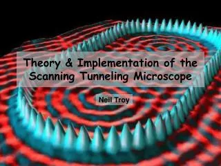
Theory & Implementation of the Scanning Tunneling Microscope. Neil Troy. The Scanning Tunneling Microscope (STM). Classical vs. Quantum mechanics Engineering Hurdles Implementation & Images.

E N D
Theory & Implementation of the Scanning Tunneling Microscope Neil Troy
The Scanning Tunneling Microscope (STM) • Classical vs. Quantum mechanics • Engineering Hurdles • Implementation & Images STM invented in 1981 by Greg Binnig & Heinrich Rohrer at IBM and were awarded with a Nobel Prize in 1986
Classical vs. Quantum Classically, if one threw a ball at a brick wall (and didn’t miss horribly) they would always find the ball on their side of the wall, because unless you are Superman there is no way that you are throwing the ball hard enough to break through the wall. Some later time Quantum mechanically, however, the ball has some finite probability of “tunneling” through the wall. The ball need not be thrown incredibly hard to achieve this, although the more energy the ball has the more likely it will be to tunnel. Some later time
Mathematical Approach Standard 1-D wave equation where U(z) is the potential of the barrier, and E is the particle’s energy Which has the normal solution of a traveling wave: where This is the general solution but in the event that U > E we can factor out an i and we get a solution that has a completely different meaning. which for our scenario, where z > 0, we get an exponential decay as the electron sees if it can tunnel through the barrier.
Visualization of tunneling Low energy particle is confined to stay in its potential well. Higher energy particle has a possibility of passing through the wall and continuing with less energy than before.
Practical application for probing A Current 0 If two metals are connected to opposite ends of a battery but are separated from each other than they logically should not conduct electricity. However, as we bring the metals extremely close to each other the wavefunctions of the electrons are able to tunnel through the gap and we will detect a current on our meter.
Let’s abandon quantum mechanics and our microscope for a second and look at the slightly different concept of arc/lightning. Only at a certain distance is the voltage going to arc through the media (air). This could be repeated and as long as the environment hasn’t changed it is very repeatable, but not practical. How this is different than arcing This is drastically different than tunneling because the extremely high voltages are physically changing the transfer medium (ionizing) so that the electrons can conduct. As such the arcing could be continuous (if the materials weren’t normally destroyed) but the current would change since the medium is constantly changing. Hi Voltage
Problems with probabilities After a little bit of math we can come up with the probability that an electron can tunnel through our barrier, where W is the barrier width. We can look at the above probability as the chance of an electron on one metal being found on the other, but likewise this works the opposite way as well. This brings rise to another problem with the above equation, even if an electron could tunnel the gap it has to have a home on the other metal. First, let’s look at biasing one movement over the gap. This is achieved just as shown previously by connecting both metals to different ends of a voltage source. This voltage is very important though, we don’t want to arc the material (high voltage) but we do want to give the electrons a natural tendency to flow one way. As such, the applied voltage is normally on the order of the work function of the material (a few eV, 4-5eV).
So many electrons to count Since we are applying a voltage nearly equivalent to the work function of the material, we are allowing any electron at, or near, the fermi energy the possibility of being free and tunneling our gap. We are now dealing with fermi energies and as such our talk must now change from individual electrons but to the masses. We now have to look at all the possible electrons that we could see tunneling our gap. Luckily, we have some bounds on these electrons, so we need not look at all of them. To be more exact we care only about a small band of electrons that are very close to the fermi energy of the material. Ef Ef-eV If we were to measure the probability as the metals are brought close we could only possibly detect those electrons move, and this is only a half truth since we still require they have a free state to tunnel into.
Currents, a more usable quantity Unfortunately, my probability meter is broken so we need some other measure of electrons moving across our gap. Electrons moving leads instantly into current so we need a way to quantify our probabilities in terms of currents. Without getting too complicated or mathematical I give you a relatively simple equation of the current we can expect to detect: where r(W,Ef) is the density of states of one metal through the gap, W, at the other metal.
Some engineering concerns With some physics in the bag let’s look at some engineering challenges. We need an extremely accurate way to bring a probing material to our sample, that is stable and is capable of very fine adjustments. To give you a feel for if one cranked out some numbers for the above equations we need to be able to bring our probe to within Angstroms of the surface and then be able to move in Angstrom increments. Sample Probe Angstroms
Some engineering concerns (cont.) A second problem is that we cannot simply move a block of metal towards a sample, if we did we would be probing the entire surface at once and that is only if our surface is perfectly flat! Sample Probe We’ll look at this one first.
Current ~e-2(6)k ~2e-2(9)k A perfect probe Hopefully, it is clear that we should have a probe that is extremely small, or ideally on the atomic scale. If we were to look at the math again (which I’m not) we would see that if we had a probe that had exactly one atom on the end then the subsequent atoms behind it would contribute almost nothing to our current. Sample 6Å 3Å As it turns out atomic probes are easily made with either mechanical or chemical processes.
Accurate distance control Angstrom level distance control is required which would be impossible for any mechanical gear workings. Enter the world of piezoelectrics A piezoelectric is a crystal that creates potential differences (voltages) when mechanical stresses are imposed on it. Voltage 0
Piezoelectric motors The mechanical to electrical effect is completely reversible and by applying voltages to these materials we force mechanical effects out of them. In fact this effect is so common place that we can find it in everyday objects like speakers to printers, and they can be as sophisticated as extremely accurate mirror control in laser laboratories. One can reliably place our sampling tip within 10’s of Angstroms from a surface without using piezoelectric motors but beyond that the accurate probing is handled by the piezoelectric. We’ll even use these motors in a feedback system to adjust the height of our probe.
PROBE Current Height Distance Distance Probing a surface With all of the elements in place we can start probing our metallic surface. We could either probe at a constant height and look at current variations as we pass. Or we could vary the height in search for constant current.
Probing a surface & what it says Although more complex, one normally modulates the height of the probe. We can see this as a major advantage in the sense that we are not contingent on the surface being very uniform, a crag or cliff of atoms does not pose a collision hazard as well as at a constant current we can suppress effects that may come with higher currents (heat, breakdown of tip, etc.). The biggest thing we must keep in mind is that an STM cannot “see” atoms. An STM probes the density of states of a surface. As such, holes are a common artifact of STM, a hole does not mean that no atom exists it merely means that the probe cannot reach below the first layer of atoms. Likewise, peaks in an STM do not necessarily mean there is a mountain of atoms, the atoms may be a different element from the surroundings and may possess a higher density of states resulting in a higher current/probe height.
Images of an STM The Nobel prize winning first STM. A more current example.
STM produced images STM image, 7 nm x 7 nm, of a single zig-zag chain of Cs atoms (red) on the GaAs(110) surface (blue). * *National Institute of Standards and Technology
Surface of platinum. IBM, Almaden Research Facility Surface of nickel. IBM, Almaden Research Facility Surface of copper. IBM, Almaden Research Facility
Ring of iron atoms on a copper blanket. IBM, Almaden Research Facility
Startling aside... In 1989, at the Almaden IBM Research Facility scientists found that an STM could be used to lift atoms off a surface of metal and placed back in a different location, at low temperatures that is.