Download
1 / 57
570 likes | 858 Vues
Learning in Bayes Nets. Task 1: Given the network structure and given data, where a data point is an observed setting for the variables, learn the CPTs for the Bayes Net. Might also start with priors for CPT probabilities.

E N D
Learning in Bayes Nets • Task 1: Given the network structure and given data, where a data point is an observed setting for the variables, learn the CPTs for the Bayes Net. Might also start with priors for CPT probabilities. • Task 2: Given only the data (and possibly a prior over Bayes Nets), learn the entire Bayes Net (both Net structure and CPTs).
Task 1: Maximum Likelihood by Example (Howard 1970) • Suppose we have a thumbtack (with a round flat head and sharp point) that when flipped can land either with the point up (tails) or with the point touching the ground (heads). • Suppose we flip the thumbtack 100 times, and 70 times it lands on heads. Then we estimate that the probability of heads the next time is 0.7. This is the maximum likelihood estimate.
The General Maximum Likelihood Setting • We had a binomial distribution b(n,p) for n=100, and we wanted a good guess at p. • We chose the p that would maximize the probability of our observation of 70 heads. • In general we have a parameterized distribution and want to estimate a (several) parameter(s): choose the value that maximizes the probability of the data.
Back to the Frequentist-Bayes Debate • The preceding seems backwards: we want to maximize the probability of p, not necessarily of the data (we already have it). • A Frequentist will say this is the best we can do: we can’t talk about probability of p; it is fixed (though unknown). • A Bayesian says the probability of p is the degree of belief we assign to it ...
Fortunately the Two Agree (Almost) • It turns out that for Bayesians, if our prior belief is that all values of p are equally likely, then after observing the data we’ll assign the highest probability to the maximum likelihood estimate for p. • But what if our prior belief is different? How do we merge the prior belief with the data to get the best new belief?
Any intuition for this? • For any positive integer y, G(y) = (y-1)!. • Suppose we use this, and we also replace • x with p • a with x • a+b with n • Then we get: • The beta(a,b) is just the binomial(n,p) where n=a+p, and p becomes the variable. With change of variable, we need a different normalizing constant so the sum (integral) is 1. Hence (n+1)! replaces n!.
Incorporating a Prior • We assume a beta distribution as our prior distribution over the parameter p. • Nice properties: unimodal, we can choose the mode to reflect the most probable value, we can choose the variance to reflect our confidence in this value. • Best property: a beta distribution is parameterized by two positive numbers, a
Beta Distribution (Continued) • (Continued)… and b. Higher values of a relative to b cause the mode of the distribution to be more to the left, and higher values of both a and b cause the distribution to be more peaked (lower variance). We might for example take a to be the number of heads, and b to be the number of tails. At any time, the mode of
Beta Distribution (Continued) • (Continued)… the beta distribution (the expectation for p) is a/(a+b), and as we get more data, the distribution becomes more peaked reflecting higher confidence in our expectation. So we can specify our prior belief for p by choosing initial values for a and b such that a/(a+b)=p, and we can specify confidence in this belief with high
Beta Distribution (Continued) • (Continued)… initial values for a and b. Updating our prior belief based on data to obtain a posterior belief simply requires incrementing a for every heads outcome and incrementing b for every tails outcome. • So after h heads out of n flips, our posterior distribution says P(heads)=(a+h)/(a+b+n).
Dirichlet Distributions • What if our variable is not Boolean but can take on more values? (Let’s still assume our variables are discrete.) • Dirichlet distributions are an extension of beta distributions for the multi-valued case (corresponding to the extension from binomial to multinomial distributions). • A Dirichlet distribution over a variable with n values has n parameters rather than 2.
Back to Frequentist-Bayes Debate • Recall that under the frequentist view we estimate each parameter p by taking the ML estimate (maximum likelihood estimate: the value for p that maximizes the probability of the data). • Under the Bayesian view, we now have a prior distribution over values of p. If this prior is a beta, or more generally a Dirichlet
Frequentist-Bayes Debate (Continued) • (Continued)… then we can update it to a posterior distribution quite easily using the data as illustrated in the thumbtack example. The result yields a new value for the parameter p we wish to estimate (e.g., probability of heads) called the MAP (maximum a posteriori) estimate. • If our prior distribution was uniform over values for p, then ML and MAP agree.
Learning CPTs from Complete Settings • Suppose we are given a set of data, where each data point is a complete setting for all the variables. • One assumption we make is that the data set is a random sample from the distribution we’re trying to model. • For each node in our network, we consider each entry in its CPT (each setting of values
Learning CPTs (Continued) • (Continued)… for its parents). For each entry in the CPT, we have a prior (possibly uniform) Dirichlet distribution over its values. We simply update this distribution based on the relevant data points (those that agree on the settings for the parents that correspond with this CPT entry). • A second, implicit assumption is that the
Learning CPTs (Continued) • (Continued)… distributions over different rows of the CPT are independent of one another. • Finally, it is worth noting that instead of this last assumption, we might have a stronger bias over the form of the CPT. We might believe it is a noisy-OR, a linear function, or a tree, in which case we would instead use machine learning, linear regression, etc.
Simple Example • Suppose we believe the variables PinLength and HeadWeight directly influence whether a thumbtack comes up heads or tails. For simplicity, suppose PinLength can be long or short and HeadWeight can be heavy or light. • Suppose we adopt the following prior over the CPT entries for the variable Thumbtack.
Simple Example (Continued) • Notice that we have equal confidence in our prior (initial) probabilities for the first and last columns of the CPT, less confidence in those of the second column, and more in those of the third column. • A new data point will affect only one of the columns. A new data point will have more effect on the second column than the others.
More Difficult Case: What if Some Variables are Missing • Recall our earlier notion of hidden variables. • Sometimes a variable is hidden because it cannot be explicitly measured. For example, we might hypothesize that a chromosomal abnormality is responsible for some patients with a particular cancer not responding well to treatment.
Missing Values (Continued) • We might include a node for this chromosomal abnormality in our network because we strongly believe it exists, other variables can be used to predict it, and it is in turn predictive of still other variables. • But in estimating CPTs from data, none of our data points has a value for this variable.
Missing Values (Continued) • This missing value (hidden variable) problem arises frequently. • Chicken-and-Egg issue: if we had CPTs, we could fill in the data, or if we had data we could estimate CPTs. • We do have partial data and partial (prior) CPTs. Can we somehow leverage these into full data and posterior CPTs?
Three Approaches • Expectation-Maximization (EM) Algorithm. • Gibbs Sampling (again). • Gradient Ascent (Hill-climbing).
General EM Framework • Given: Data with missing values, Space of possible models, Initial model. • Repeat until no change greater than threshold: • Expectation (E) Step: Compute expectation over missing values, given model. • Maximization (M) Step: Replace current model with model that maximizes probability of data.
(“Soft”) EM vs. “Hard” EM • Standard (soft) EM: expectation is a probability distribution. • Hard EM: expectation is “all or nothing”… most likely/probable value. • K-means is usually run as “hard” EM but doesn’t have to be. • Advantage of hard EM is computational efficiency when expectation is over state consisting of values for multiple variables (next example illustrates).
EM for Parameter Learning: E Step • For each data point with missing values, compute the probability of each possible completion of that data point. Replace the original data point with all these completions, weighted by probabilities. • Computing the probability of each completion (expectation) is just answering query over missing variables given others.
EM for Parameter Learning: M Step • Use the completed data set to update our Dirichlet distributions as we would use any complete data set, except that our counts (tallies) may be fractional now. • Update CPTs based on new Dirichlet distributions, as we would with any complete data set.
EM for Parameter Learning • Iterate E and M steps until no changes occur. We will not necessarily get the global MAP (or ML given uniform priors) setting of all the CPT entries, but under a natural set of conditions we are guaranteed convergence to a local MAP solution. • EM algorithm is used for a wide variety of tasks outside of BN learning as well.
Subtlety for Parameter Learning • Overcounting based on number of interations required to converge to settings for the missing values. • After each repetition of E step, reset all Dirichlet distributions before repeating M step.
EM for Parameter Learning Data P(A) 0.1 (1,9) P(B) 0.2 (1,4) A B • A B C D E • 0 0 ? 0 0 • 0 0 ? 1 0 • 0 ? 1 1 • 0 0 ? 0 1 • 0 1 ? 1 0 • 0 0 ? 0 1 • 1 ? 1 1 • 0 0 ? 0 0 • 0 0 ? 1 0 • 0 0 ? 0 1 A B P(C) T T 0.9 (9,1) T F 0.6 (3,2) F T 0.3 (3,7) F F 0.2 (1,4) C E D C P(E) T 0.8 (4,1) F 0.1 (1,9) C P(D) T 0.9 (9,1) F 0.2 (1,4)
P(A) 0.1 (1,9) • A B C D E • 0 0 0 0 • 0 0 1 0 • 0 1 1 • 0 0 0 1 • 0 1 1 0 • 0 0 0 1 • 1 1 1 • 0 0 0 0 • 0 0 1 0 • 0 0 0 1 EM for Parameter Learning Data P(B) 0.2 (1,4) A B 0: 0.99 1: 0.01 A B P(C) T T 0.9 (9,1) T F 0.6 (3,2) F T 0.3 (3,7) F F 0.2 (1,4) 0: 0.80 1: 0.20 0: 0.02 1: 0.98 C 0: 0.80 1: 0.20 0: 0.70 1: 0.30 0: 0.80 1: 0.20 E D 0: 0.003 1: 0.997 C P(E) T 0.8 (4,1) F 0.1 (1,9) C P(D) T 0.9 (9,1) F 0.2 (1,4) 0: 0.99 1: 0.01 0: 0.80 1: 0.20 0: 0.80 1: 0.20
P(A) 0.1 (1,9) Multiple Missing Values Data P(B) 0.2 (1,4) A B C D E ? 0 ? 0 1 A B A B P(C) T T 0.9 (9,1) T F 0.6 (3,2) F T 0.3 (3,7) F F 0.2 (1,4) C E D C P(E) T 0.8 (4,1) F 0.1 (1,9) C P(D) T 0.9 (9,1) F 0.2 (1,4)
P(A) 0.1 (1,9) C P(D) T 0.9 (9,1) F 0.2 (1,4) Multiple Missing Values Data P(B) 0.2 (1,4) A B C D E 0 0 0 0 1 0 0 1 0 1 1 0 0 0 1 1 0 1 0 1 A B 0.72 0.18 0.04 0.06 A B P(C) T T 0.9 (9,1) T F 0.6 (3,2) F T 0.3 (3,7) F F 0.2 (1,4) C E D C P(E) T 0.8 (4,1) F 0.1 (1,9)
Data A B C D E 0 0 0 0 1 0 0 1 0 1 1 0 0 0 1 1 0 1 0 1 0.72 0.18 0.04 0.06 Multiple Missing Values P(A) 0.1 (1.1,9.9) P(B) 0.17 (1,5) A B A B P(C) T T 0.9 (9,1) T F 0.6 (3.06,2.04) F T 0.3 (3,7) F F 0.2 (1.18,4.72) C E D C P(E) T 0.81 (4.24,1) F 0.16 (1.76,9) C P(D) T 0.88 (9,1.24) F 0.17 (1,4.76)
Problems with EM • Only local optimum (not much way around that, though). • Deterministic … if priors are uniform, may be impossible to make any progress… • … next figure illustrates the need for some randomization to move us off an uninformative prior…
P(A) 0.5 (1,1) B P(C) T 0.5 (1,1) F 0.5 (1,1) A P(B) T 0.5 (1,1) F 0.5 (1,1) What will EM do here? Data A • A B C • 0 ? 0 • ? 1 • 0 ? 0 • ? 1 • 0 ? 0 • 1 ? 1 B C
P(A) 0.5 (1,1) B P(C) T 0.5 (1,1) F 0.5 (1,1) A P(B) T 0.6 (6,4) F 0.4 (4,6) EM Dependent on Initial Beliefs Data A • A B C • 0 ? 0 • ? 1 • 0 ? 0 • ? 1 • 0 ? 0 • 1 ? 1 B C
P(A) 0.5 (1,1) B P(C) T 0.5 (1,1) F 0.5 (1,1) A P(B) T 0.6 (6,4) F 0.4 (4,6) EM Dependent on Initial Beliefs B is more likely T than F when A is T. Filling this in makes C more likely T than F when B is T. This makes B still more likely T than F when A is T. Etc. Small change in CPT for B (swap 0.6 and 0.4) would have opposite effect. Data A • A B C • 0 ? 0 • ? 1 • 0 ? 0 • ? 1 • 0 ? 0 • 1 ? 1 B C
A Second Approach: Gibbs Sampling • The idea is analogous to Gibbs Sampling for Bayes Net inference, which we have seen in detail. • First, initialize the values of hidden variables arbitrarily. Update CPTs based on current (now complete) data. • Second, choose one data point and one unobserved variable X for that data point.
Gibbs Sampling (Continued) • (Continued)… Reset the value of X within that data point based on the current CPTs and the current setting of the variables in the Markov Blanket of X within that data point. • Third, repeat this process for all the other unobserved variables throughout the data set and then update the CPTs.
Gibbs Sampling (Continued) • Fourth, iterate through the previous three steps some number of times (chain length) • Gibbs faster than (soft) EM if many data missing values per data point. • Gibbs often slower than hard EM (we have more variables now than in the inference case) but results may be better.
Approach 3: Gradient Ascent • We want to maximize posterior probability (or likelihood if uniform priors). Where w1,…,wk are the probabilities in the CPTs (analogous to weights in a neural network) and D1,…, Dn are the data points, we will use a greedy hill-climbing search (making small changes in the direction of the gradient) to maximize P(D|w1,…,wk) = P(D1|w1,…,wk)...P(Dn|w1,…,wk).