Download
1 / 26
280 likes | 525 Vues
Exact Inference in Bayes Nets. Inference Techniques. Exact Inference Variable elimination Belief propagation ( polytrees ) Junction tree algorithm (arbitrary graphs) Kalman filte Adams & MacKay changepoint Approximate Inference Loopy belief propagation Rejection sampling

E N D
Inference Techniques • Exact Inference • Variable elimination • Belief propagation (polytrees) • Junction tree algorithm (arbitrary graphs) • Kalmanfilte • Adams & MacKay changepoint • Approximate Inference • Loopy belief propagation • Rejection sampling • Importance sampling • Markov Chain Monte Carlo (MCMC) • Gibbs sampling • Variational approximations • Expectation maximization (forward-backward algorithm) • Particle filters Later in the semester
Notation • U: set of nodes in a graph • Xi: random variable associated with node i • πi: parents of node i • Joint probability: General form to include undirectedas well as directed graphs: • where C is an index over cliques • to apply to directed graph, turn directed graph into moral graph • moral graph: connect all parents of each node and remove arrows
Common Inference Problems • Assume partition of graph into subsets • O = observations; U = unknowns; N = nuisance variables • Computing marginals (avg. over nuisance vars.) • Computing MAP probability • Given observations O, find distribution over U
Variable Elimination • E.g., calculating marginal p(x5) • Elimination order: 1, 2, 4, 3 m43(x3) m12(x2) m23(x3) m35(x5)
Variable Elimination • E.g., calculating conditional p(x5|x2,x4) m43(x3) m12(x2) m23(x3) m35(x5)
Quiz: Variable Elimination • Elimination order for P(C)? • Elimination order for P(D) ? A B C D E
What If Wrong Order Is Chosen? • Compute P(B) with order D, E, C, A • Compute P(B) with order A, C, D, E A B C D E
Weaknesses Of Variable Elimination • 1. Efficiency of algorithm strongly dependent on choosing the best elimination order • NP-hard problem • 2. Inefficient if you want to compute multiple queries conditioned on the same evidence.
Message Passing • Inference as elimination process → • Inference as passing messages along edges of (moral) graph • Leads to efficient inference when you want to make multiple inferences, because each message can contribute to more than one marginal.
Message Passing • mij(xj): intermediate term • i is variable being summed over, j is other variable • Note dependence on elimination ordering
What are these messages? • Message from Xi to Xj says, • “Xi thinks that Xj belongs in these states with various likelihoods.” • Messages are similar to likelihoods • non-negative • Don’t have to sum to 1, but you can normalize them without affecting results (which adds some numerical stability) • large message means that Xi believes that the marginal value of Xj=xj with high probability • Result of message passing is a consensus that determines the marginal probabilities of all variables
Belief Propagation (Pearl, 1983) • i: node we're sending from • j: node we're sending to • N(i): neighbors of i • N(i)\j: all neighbors of i excluding j • e.g., • computing marginal probability:
Belief Propagation (Pearl, 1983) i: node we're sending from j: node we're sending to • Start with i = leaf nodes of undirectedgraph (nodes with one edge) N(i)\j = Ø • Tree structure guarantees each node ican collect messages from all N(i)\j before passing message on to j
Computing MAP Probability • Same operation with summation replaced by max
Polytrees • Can do exact inference via belief propagation and variable elimination for polytrees • Polytree • Directed graph with at most one undirectedpath between two vertices • DAG with no undirected cycles • If there were undirected cycles, messagepassing would produce infinite loops
Efficiency of Belief Propagation • With trees, BP terminates after two steps • 1 step to propagate information from outside in • 1 step to propagate information from inside out • boils down to calculation like variable elimination over all eliminations • With polytrees, belief propagation converges in time • linearly related to diameter of net • but multiple iterations are required (not 1 pass as for trees) • polynomial In number of states of each variable
Inference Techniques • Exact Inference • Variable elimination • Belief propagation (polytrees) • Junction tree algorithm (arbitrary graphs) • Kalmanfilte • Adams & MacKay changepoint • Approximate Inference • Loopy belief propagation • Rejection sampling • Importance sampling • Markov Chain Monte Carlo (MCMC) • Gibbs sampling • Variational approximations • Expectation maximization (forward-backward algorithm) • Particle filters Later in the semester
Junction Tree Algorithm Works for general graphs • not just trees but also graphs with cycles • both directed and undirected • Basic idea • Eliminate cycles by clustering nodes into cliques • Perform belief propagation on cliques Exact inference of (clique) marginals
Junction Tree Algorithm 1. Moralization • If graph is directed, turn it into an undirected graph by linking parents of each node and dropping arrows 2. Triangulation • Decide on elimination order. • Imagine removing nodes in order and adding a link between remaining neighbors of node i when node i is removed. • e.g., elimination order (5, 4, 3, 2)
Junction Tree Algorithm 3. Construct the junction tree • one node for every maximal clique • form maximal spanning tree of cliques • clique tree is a junction tree if for every pair of cliques V and W, then all cliques on the (unique) path between V and W contain V∩W • If this property holds, then local propagation of information will lead to global consistency.
Junction Tree Algorithm This is a junction tree. This is not a junction tree.
Junction Tree Algorithm 4. Transfer the potentials from original graph to moral graph • define a potential for each clique, ψC(xC)
Junction Tree Algorithm 5. Propagate • Given junction tree and potentials on the cliques, can send messages from clique Ci to Cj • Sij: nodes shared by i and jN(i): neighboring cliques of i • Messages get sent in all directions. • Once messages propagated, can determine the marginal prob of any clique.
Computational Complexityof Exact Inference Exponential in number of nodes in a clique • need to integrate over all nodes Goal is to find a triangulation that yields the smallest maximal clique • NP-hard problem →Approximate inference
Loopy Belief Propagation • Instead of making a single pass from the leaves, perform iterative refinement of message variables. • initialize all variables to 1 • recompute all variables assuming the values of the other variables • iterate until convergence • For polytrees, guaranteed to converge in time ~ longest undirected path through tree. • For general graphs, some sufficiency conditions, and some graphs known not to converge.