Download
1 / 81
810 likes | 844 Vues
Delve into the fundamentals of probability and Bayes Nets to enhance reasoning and decision-making skills. Learn about conditional probabilities, joint distributions, and exploiting conditional independence in Bayesian networks.

E N D
Probability • The world is a very uncertain place. • As of this point, we’ve basically danced around that fact. We’ve assumed that what we see in the world is really there, what we do in the world has predictable outcomes, etc.
C B A Some limitations we’ve encountered so far ... move(A,up) = B move(A,down) = C In the search algorithms we’ve explored so far, we’ve assumed a deterministic relationship between moves and successors
A B C Some limitations we’ve encountered so far ... 0.5 move(A,up) = B 50% of the time move(A,up) = C 50% of the time 0.5 Lots of problems aren’t this way!
A B C Some limitations we’ve encountered so far ... Based on what we see, there’s a 30% chance we’re in A, 30% in B and 40% in C .... Moreover, lots of times we don’t know exactly where we are in our search ...
How to cope? • We have to incorporate probability into our graphs, to help us reason and make good decisions. • This requires a review of probability basics.
Boolean Random Variable • A boolean random variable is a variable that can be true or false with some probability. • A = The next president is a liberal. • A = You wake up tomorrow with a headache. • A = You have the flu.
Visualizing P(A) • Call P(A) as “the fraction of possible worlds in which A is true”. Let’s visualize this:
The axioms of probability • 0 <= P(A) <= 1 • P(True) = 1 • P(False) = 0 • P(A or B) = P(A) + P(B) - P(A and B) • We will visualize each of these axioms in turn.
Theorems from the axioms • 0 <= P(A) <= 1 • P(True) = 1 • P(False) = 0 • P(A or B) = P(A) + P(B) - P(A and B) • From these we can prove:P(not A) = P(~A) = 1-P(A).
Reasoning with Conditional Probability One day you wake up with a headache. You think: “Drat! 50% of flu cases are associated with headaches so I must have a 50-50 chance of coming down with flu”. Is that good reasoning?
Using Bayes Rule to gamble Trivial question: Someone picks an envelope and random and asks you to bet as to whether or not it holds a dollar. What are your odds?
Using Bayes Rule to gamble Not trivial question: Someone lets you take a bead out of the envelope before you bet. If it is black, what are your odds? If it is red, what are your odds?
Joint Distributions Boolean variables A, B and C • A joint distribution records the probabilities that multiple variables will hold particular values. They can be represented much like truth tables. • They can be populated using expert knowledge, by using the axioms of probability, or by actual data. • Note that the sum of all the probabilities MUST be 1, in order to satisfy the axioms of probability.
Note: these probabilities are from the UCI “Adult” Census, which you, too, can fool around with in your leisure ....
Where we are • We have been learning how to make inferences. • I’ve got a sore neck: how likely am I to have the flu? • The polls have a liberal president ahead by 5 points: how likely is he or she to win the election? • This person is reading an email about guitars: how likely is he or she to want to buy guitar picks? • This is a big deal, as inference is at the core of a lot of industry. Predicting polls, the stock market, optimizing ad placements, etc., can potentially earn you money. Predicting a flu outbreak, moreover, can help the world (because, after all, money is not everything).
Independence • The census data is represented as vectors of variables, and the occurrence of values for each variable has a certain probability. • We will say that variables like {gender} and {hrs worked per week} are independent if and only if: • P(hours worked | gender) = P(hours worked) • P(gender | hours worked) = P(gender)
Conditional independence These pictures represent the probabilities of events A, B and C by the areas shaded red, blue and yellow respectively with respect to the total area. In both examples A and B are conditionally independent given C because: P(A^B| C) = P(A|C)P(B|C) BUT A and B are NOT conditionally independent given ~C, as: P(A^B|~ C) != P(A|~C)P(B|~C)
The Value of Independence • Complete independence reduces both representation of joint and inference from O(2n) to O(n)! • Unfortunately, such complete mutual independence is very rare. Most realistic domains do not exhibit this property. • Fortunately, most domains do exhibit a fair amount of conditional independence. And we can exploit conditional independence for representation and inference as well. • Bayesian networks do just this.
C H A B E Exploiting Conditional Independence • Let’s see what conditional independence buys us. • Consider a story: • “If Craig woke up too early (E is true), Craig probably needs coffee (C); if Craig needs coffee, he's likely angry (A). If he is angry, he has an increased chance of bursting a brain vessel (B). If he bursts a brain vessel, Craig is quite likely to be hospitalized (H).” E – Craig woke too early A – Craig is angry H – Craig hospitalized C – Craig needs coffee B – Craig burst a blood vessel
C H A B E Cond’l Independence in our Story • If you knew E, C, A, or B, your assessment of P(H) would change. • E.g., if any of these are seen to be true, you would increase P(H) and decrease P(~H). • This means H is not independent of E, or C, or A, or B. • If you knew B, you’d be in good shape to evaluate P(H). You would not need to know the values of E, C, or A. The influence these factors have on H is mediated by B. • Craig doesn't get sent to the hospital because he's angry, he gets sent because he's had an aneurysm. • So H is independent of E, and C, and A, given B
C H A B E Cond’l Independence in our Story • Similarly: • B is independent of E, and C, given A • A is independent of E, given C • This means that: • P(H | B, {A,C,E} ) = P(H|B) • i.e., for any subset of {A,C,E}, this relation holds • P(B | A, {C,E} ) = P(B | A) • P(A | C, {E} ) = P(A | C) • P(C | E) and P(E) don’t “simplify”
C H A B E Cond’l Independence in our Story • By the chain rule (for any instantiation of H…E): • P(H,B,A,C,E) = • P(H|B,A,C,E) P(B|A,C,E) P(A|C,E) P(C|E) P(E) • By our independence assumptions: • P(H,B,A,C,E) = • P(H|B) P(B|A) P(A|C) P(C|E) P(E) • We can specify the full joint by specifying five local conditional distributions (joints): P(H|B); P(B|A); P(A|C); P(C|E); and P(E)
C H A B E Example Quantification P(B|A) = 0.2 P(~B|A) = 0.8 P(B|~A) = 0.1 P(~B|~A) = 0.9 P(C|E) = 0.8 P(~C|E) = 0.2 P(C|~E) = 0.5 P(~C|~E) = 0.5 • Specifying the joint requires only 9 parameters (if we note that half of these are “1 minus” the others), instead of 31 for explicit representation • That means inference is linear in the number of variables instead of exponential! • Moreover, inference is linear generally if dependence has a chain structure P(A|C) = 0.7 P(~A|C) = 0.3 P(A|~C) = 0.0 P(~A|~C) = 1.0 P(H|B) = 0.9 P(~H|B) = 0.1 P(H|~B) = 0.1 P(~H|~B) = 0.9 P(E) = 0.7 P(~E) = 0.3
C H A B E Inference • Want to know P(A)? Proceed as follows: These are all terms specified in our local distributions!
Bayesian Networks • The structure we just described is a Bayesian network. A BN is a graphical representation of the direct dependencies over a set of variables, together with a set of conditional probability tables quantifying the strength of those influences. • Bayes nets generalize the above ideas in very interesting ways, leading to effective means of representation and inference under uncertainty.
Let’s do another Bayes Net example with different instructors M: Maryam leads tutorial S: It is sunny out L: The tutorial leader arrives late Assume that all tutorial leaders may arrive late in bad weather. Some leaders may be more likely to be late than others.
Bayes net example • M: Maryam leads tutorial • S: It is sunny out • L: The tutorial leader arrives late • Because of conditional independence, we only need 6 values in the joint instead of 7. Again, conditional independence leads to computational savings!
Bayes net example • M: Maryam leads tutorial • S: It is sunny out • L: The tutorial leader arrives late
Read the absence of an arrow between S and M to mean “It would not help me predict M if I knew the value of S” Read the two arrows into L to mean “If I want to know the value of L it may help me to know M and to know S.”
Adding to the graph • Now let’s suppose we have these three events: • M: Maryam leads tutorial • L: The tutorial leader arrives late • R : The tutorial concerns Reasoning with Bayes’ Nets • And we know: • Abdel-rahman has a higher chance of being late than Maryam. • Abdel-rahman has a higher chance of giving lectures about reasoning with BNs • What kind of independences exist in our graph?
Conditional independence, again Once you know who the lecturer is, then whether they arrive late doesn’t affect whether the lecture concerns Reasoning with Bayes’ Nets.
Let’s assume we have 5 variables • M: Maryam leads tutorial • L: The tutorial leader arrives late • R:The tutorial concerns Reasoning with BNs • S: It is sunny out • T: The tutorial starts by 10:15 • We know: • T is only directly influenced by L (i.e. T is conditionally independent of R,M,S given L) • L is only directly influenced by M and S (i.e. L is conditionally independent of R given M & S) • R is only directly influenced by M (i.e. R is conditionally independent of L,S, given M) • M and S are independent
M: Maryam leads tutorial L: The tutorial leader arrives late R : The tutorial concerns Reasoning in FOL S: It is sunny out T: The tutorial starts by 10:15 Let’s make a Bayes Net Step One: add variables. • Just choose the variables you’d like to be included in the net.
M: Maryam leads tutorial L: The tutorial leader arrives late R : The tutorial concerns Reasoning in FOL S: It is sunny out T: The tutorial starts by 10:15 Making a Bayes Net Step Two: add links. • The link structure must be acyclic. • If node X is given parents Q1,Q2,..and Qn, you are promising that any variable that’s a non-descendent of X is conditionally independent of X given {Q1,Q2,..and Qn}