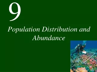
Population Distribution and Abundance
600 likes | 1.41k Vues
Population Distribution and Abundance. 8 Population Distribution and Abundance. Case Study: From Kelp Forest to Urchin Barren Populations Distribution and Abundance Geographic Range Dispersion within Populations Estimating Abundances and Distributions Case Study Revisited

Population Distribution and Abundance
E N D
Presentation Transcript
8 Population Distribution and Abundance • Case Study: From Kelp Forest to Urchin Barren • Populations • Distribution and Abundance • Geographic Range • Dispersion within Populations • Estimating Abundances and Distributions • Case Study Revisited • Connections in Nature: From Urchins to Ecosystems
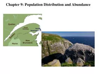
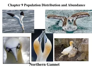
Case Study: From Kelp Forest to Urchin Barren Waters surrounding the Aleutian Islands have abundant marine life, including the sea otter. Figure 8.1 Key Players in the Forests of the Deep
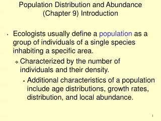
Introduction Distribution: Geographic area over which individuals of a species occur. Abundance: The number of individuals in a specific area.
Populations Concept 8.1: Populations are dynamic entities that vary in size over time and space. Population: Group of individuals of the same species that live within a particular area and interact with one another. Abundance can be reported as population size (# individuals), or density (# individuals per unit area).
Populations Example: On a 20-hectare island there are 2,500 lizards. Population size = 2,500 Population density = 125/hectare
Populations Populations may exist in patches that are spatially isolated but linked by dispersal. For example, heathlands in England have been fragmented by human development.
Populations What is an individual? Aspen trees can produce clones (genetically identical copies of themselves) by forming new plants from root buds. A grove of aspens may all be from the same individual.
Populations Other plants form clones on horizontal stems or “runners.” Animals such as corals, bryozoans, and sea anemones can also form clones. Some insects, fish, frogs, and lizards also produce clones. How can one count individuals in such a population?
Populations – Ramet vs. Genet Ramet - an ecological unit; ecologically considered an individual unit because it is mostly autonomous with regard to utilization of resources, even though it is physically connected to one or more individuals of the exact same species and identical genetic background; essentially a clone. Ex. The Aspen “Tree” Genet - a genetically distinct unit, all the tissue that grows from a single fertilized egg. A genet may encompass many ramets including ramets that are no longer connected to one another. Ex. The Aspen Grove
Distribution and Abundance Creosote bush has a broad range of distribution in North American deserts. Saguaro cactus has a more limited distribution—it can tolerate dry conditions, but not cold temperatures. Concept 8.2: The distributions and abundances of organisms are limited by habitat suitability, historical factors, and dispersal.
Figure 8.9 Joint Effects of Temperature and Competition on Barnacle Distribution
Distribution and Abundance Evolutionary history, dispersal abilities, and geologic events all affect the modern distribution of species. Example: Polar bears evolved from brown bears in the Arctic. Why are they not in the Antarctic? Penguins?
Distribution and Abundance Continental drift explains the distributions of some species. Wallace (1860) observed that animals can vary considerably over very short distances, a phenomenon that could not be explained until continental drift was proposed.
Figure 8.10 Continental Drift Affects the Distribution of Organisms
Distribution and Abundance Dispersal limitation can prevent species from reaching areas of suitable habitat. Example: The Hawaiian Islands have only one native mammal, the hoary bat, which was able to fly there.
Figure 8.11 Populations Can Expand after Experimental Dispersal
Geographic Range There is much variation in the size of geographic ranges—the entire geographic region over which a species is found. Concept 8.3: Many species have a patchy distribution of populations across their geographic range.
Geographic Range Devil’s Hole pupfish lives in a single desert pool (7 ´ 3 m across and 15 m deep). Many tropical plants have a small geographic range. In 1978, 90 new species were discovered on a single mountain ridge in Ecuador, each species was restricted to that ridge.
Geographic Range Other species, such as the coyote, have very large geographic ranges. Some species are found on several continents. Few species are found on all continents except humans, Norway rats, and the bacterium E. coli.
Figure 8.14 Populations Often Have a Patchy Distribution (Part 1)
Figure 8.14 Populations Often Have a Patchy Distribution (Part 2)
Figure 8.15 Abundance Varies Throughout a Species’ Geographic Range
Dispersion within Populations Dispersion is the spatial arrangement of individuals within a population: Regular—individuals are evenly spaced. Random—individuals scattered randomly. Clumped—the most common pattern. Concept 8.4: The dispersion of individuals within a population depends on the location of essential resources, dispersal, and behavioral interactions.
Figure 8.17 Territorial Behavior Affects Dispersion within Populations (Part 1)
Figure 8.17 Territorial Behavior Affects Dispersion within Populations (Part 2)
Estimating Abundances and Distributions Complete counts of individual organisms in a population are often difficult or impossible. Several methods are used to estimate the actual or absolute populationsize. Concept 8.5: Population abundances and distributions can be estimated with area-based counts, mark–recapture methods, and niche modeling.
Figure 8.18 Estimating Absolute Population Size Using Quadrats
Estimating Abundances and Distributions Example: 40, 10, 70, 80, and 50 chinch bugs are counted in five 10 cm ´ 10 cm (0.01 m2) quadrats.
Estimating Abundances and Distributions Mark–recapture methods are used for mobile organisms. A subset of individuals is captured and marked or tagged in some way, then released. At a later date, individuals are captured again, and the ratio of marked to unmarked individuals is used to estimate population size.
Estimating Abundances and Distributions Example: 23 butterflies are captured and marked (M). Several days later, 15 are captured (C), 4 of them marked (R for recaptured). To estimate total population size (N): or
Estimating Abundances and Distributions Sometimes the available data can only provide an index of population size that is related to actual population size in unknown ways. For example number of cougar tracks in an area, or number of fish caught per unit of effort.
Estimating Abundances and Distributions These data can be compared from one time period to another, allowing an estimate of relative population size. Interpretation is tricky (e.g. the number of cougar tracks is related to population density, but also activity levels of individuals).
Figure 8.19 Causing the Outbreak? From Rain to Plants to Mice
Case Study Revisited: From Kelp Forest to Urchin Barren Do sea urchins starve after kelp forests have disappeared? Urchins are able to survive on other foods—other algae, benthic diatoms, and detritus (recently dead or partly-decomposed organisms). They can also reduce their metabolic rate, reabsorb sex organs, and absorb dissolved nutrients directly from seawater.
Figure 8.22 Orca Predation on Otters May Have Led to Kelp Decline (Part 1)
Figure 8.22 Orca Predation on Otters May Have Led to Kelp Decline (Part 2)
Connections in Nature: From Urchins to Ecosystems Kelp forests have strong effects on nearshore ecosystems. They are very productive, rivaling tropical rainforests for biomass production. The tips of the kelp fronds are constantly eroding, creating floating detritus which is food for many organisms.