Boundary Layer Notes 5
Boundary Layer Notes 5. Observational Techniques. Observational Techniques. Sources: Kaimal & Finnegan, Atmospheric Boundary Layer Flows: their structure and measurement, Oxford University Press, 1994 In situ techniques: Important boundary layer measurements:

Boundary Layer Notes 5
E N D
Presentation Transcript
Boundary Layer Notes 5 • Observational Techniques
Observational Techniques Sources: Kaimal & Finnegan, Atmospheric Boundary Layer Flows: their structure and measurement, Oxford University Press, 1994 • In situ techniques: • Important boundary layer measurements: T, u, v, w, q, trace gases (e.g. CO2, CH4)
Observational Techniques We need to measure both mean quantities and fluctuations. • Why fluctuations? After all we can use flux-gradient relationships to determine fluxes using mean conditions. Answer: because we don’t know if we can trust the flux-gradient relationships; especially in very turbulent, nearly well-mixed boundary layers.
For means, standard measurement techniques are acceptable (thermistors, wind vanes, cup-anemometers, propellers, hygristors, psychrometer, dew-point hygrometer) • Sketch dew-point hygrometer, psychrometer.
For fluctuations, we need to get more clever. • Why? Response time. We need independent measurements every 0.1 s to produce reliable flux measurements. • Solution: sonic anemometers, sonic thermometers, and TDL (and other radiometric) observations of trace gases. • How do sonic anemometers work? • Derive speed of sound c = √gamma RTv/m • Note approximateness of Tv dependence… derive (1 + 0.38e/p) factor…. • Sketch sonic anemometer layout, to justify Vd = c2/2d*(t2-t1), • (old fashioned measurement, when anemometer only measures the difference between the times). • Vd = d/2*(1/t1 – 1/t2) • Mast issues… have to place instruments far away, and not down-wind of towers.
Remote sensing—fine for mean state of boundary layer, not for direct flux measurements. • Describe • radar wind profiles • Sodar • Lidar • Radio Acoustic Sounding System (bouncing radar off of density gradients caused by sound wave emissions).(lidar very expensive as of ’94 anyway). • Old wind profilers weren’t useful for boundary layer studies because their minimum ranges were ~1 km. Newer ones at 915 Mhz can measure from 100 m to 1.5 km + with 50 m resolution. But time constant is still ~a few minutes.
Sonic Anemometer Derive speed of sound: Sketch anemometer layout, and derive:
Sonic Anemometer, cont’d. • We can now make our measurement of the temperature more accurate, by adding together the reciprocals of the separate times, and if we’re using a three-dimensional sonic anemometer, we can get t1 and t2 from the vertical anemometer axis, and Vn from the magnitude of the horizontal wind.
A bunch of sonic anemometers from Applied Technologies. Data rates range from 10/s to 1/s.f
Li-Cor (brand) IR absorbtion Gas Analyzers. Funny-looking one is an open cell, for eddy-correlation measurements.