Example 1
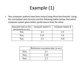
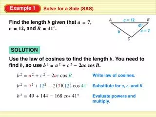
Example 1 To predict the asking price of a used Chevrolet Camaro, the following data were collected on the car’s age and mileage. Data is stored in CAMARO1. Determine the regression equation and answer additional questions stated later. Solution

Example 1
E N D
Presentation Transcript
Example 1 • To predict the asking price of a used Chevrolet Camaro, the following data were collected on the car’s age and mileage. Data is stored in CAMARO1.Determine the regression equation and answer additional questions stated later. • Solution • Run the regression tool from Excel > Data analysis. Click to see the output next
The regression equation The regression equation: Price =17499.1-1131.64Age-72.31MileageBe careful about the interpretation of the intercept (17499).Do not argue that this is the price of a used car with no mileagewhen its age is “zero”. Although such cars may exist (a car purchased and returned within a week with almost no mileage)might need to be re-sold as a used car. Yet, such values of Age and Mileage were not covered by the sample range!!. CAMARO1
The model usefulness CAMARO1 • Does the overall model contribute significantly to predicting the asking price of a used Chevrolet Camaro? Use .01 for the significance level Answer:Observe the Significance F. This is the p value for the F Test of the hypothesesH0: b1= b2 = 0H1: At least one b ¹0. Since the p value is practically zero, it is smaller than alpha. The null hypothesis is rejected, and therefore at least one b ¹0. The variable associated with this b is linearly related to the price, and the model is useful, thus contributes to predicting the asking price.
Model’s fit • How well does the model fit the data? Would you expect the predictions to be accurate with this model? • Solution • Observing the coefficient of determination (R2), 81% of the variation in car prices are explained by this model. This is quite high, and we can expect accurate predictions.
Predicting ‘y’ • Predict the value of the asking price for a 5-years old car, with 70,000 miles on the odometer, with 95% confidence. • Solution • To obtain an interval estimate for the prediction of a single car asking price when Age=5, and Mileage=70, we look for the prediction interval. From Data Analysis Plus we have {$2622.222, $10936.38}. • The general form of the interval is: , where D is determined from the data.Specifically: 17499.1-1131.64(5)-72.31(70)= 6779.303.So the interval is 6779.303± D, For the Data Analysis Plus procedure go to the worksheet “Prediction Interval” in “CAMARO1”.
Estimating the mean ‘y’ • Predict the value of the mean asking price for all 5-years old cars, with 70,000 miles on the odometer, with 95% confidence. • Solution • To obtain an interval estimate for the mean asking price of all cars for which Age=5 and Mileage=70, we look for the confidence interval. From Data Analysis Plus we have {$5756.028, $7802.577}For details go to the worksheet “Prediction Interval” in “CAMARO1”.
Testing linear relationship • Are both variables (Age and Mileage each one in the presence of the other one), serve as good predictors of Asking Price? Test at alpha=.025. • Solution • Perform a t-test for the b coefficient of each variable. The hypotheses tested are: H0: bAge=0 vs. H1: bAge¹ 0 for which the p value is .002; H0: bMileage=0 vs. H1: bMileage¹ 0 for which the p value is .0104. In both cases the null hypothesis is rejected, therefore, both have linear relationship to the asking price at 2.5% significance level.
Problem 2 • The previous model for the prediction of the asking price of used Chevrolet Camaro, is now extended by adding two new independent variables: car condition (Excellent, Average, Poor), and the type of the seller who sells the car (Dealer, Individual). The data for this case is stored in CAMARO2 (see next slide). • Develop the linear regression model for this case and answer several questions formulated next. • Solution • The two new variables describe the values of qualitative data (the state of a car and the type of the seller). Thus, they are dummy variables, take on the values ‘0’ and ‘1’.
Using dummy variables • Solution – continued: • There are three possible car condition values, so we need two dummy variables. Let us select the variables ‘Average’ and ‘Poor’. • In describing the two values of the car condition, these variables are used as follows: AveragePoor • An “Excellent condition” car 0 0 • An “Average condition” car 1 0 • A “Poor condition” car 0 1 • In a similar manner we use one dummy variable to describe who sold the car. Let us define Dealer = 1 if the car was sold by a dealer. Dealer = 0 if sold by an individual. CAMARO2
The linear regression equation The linear regression equation:Price= 17357.38-1131.93Age-33.242Mileage- -2556.44Avg-3275.3Poor+775.64Dealer
Interpreting the coefficients bi • Interpret the coefficient estimates bi of each variable and test the strength of their predicting power. • Solution bAge= -1131.93. In this model, For each additional year the asking price drops by $1132, keeping the rest of the variables unchanged. bMile= -33.24. In this model, for each additional 1000 miles the asking price drops by $33.24, keeping the rest of the variables unchanged. bAvg = -2556.44. In this model, the asking price for a car whose condition is average is $2556.44 lower than the asking price for a car whose condition is excellent, keeping the rest of the variables unchanged. bPoor = -3275.3. In this model, the asking price for a car whose condition is poor is $3275.3 lower than the asking price for a car whose condition is excellent, keeping the rest of the variables unchanged. bDeal = 775.64. In this model the asking price for a car sold by a dealer is $775.64 higher than this sold by an individual, keeping the rest of the variables unchanged.
The role of the dummy variable coefficients • Let us compare the asking price equations of two cars, with the same age, mileage, and condition, one sold by a dealer, the other one by an individual:Price(Dealer)=b0+b1Age+b2Mileage+b3Avg.+b4Poor +b5(Dealer=1)= b0+b1Age+b2 Mileage+b3Avg.+b4Poor +b5Price(Individual)=b0+b1Age+b2Mileage+b3Avg.+b4Poor +b5(Dealer=0)= b0+b1Age+b2Mileage+b3Avg.+b4Poor • Conclusion: When the only difference between cars is the type of sellers who sell them, the base line equation was selected to be the Price(Individual) equation, and then b5 is the average difference in asking price between them.
The role of the dummy variable coefficients • Let us compare the asking price equations of three cars, that differ in their overall condition but have the same age, mileage, and are sold by the same type of a seller:Price(Excellent)=b0+b1Age+b2 Mileage+b3(Avg.=0)+b4(Poor=0) +b5(Dealer)=b0+b1Age+b2 Mileage+b5(Dealer)Price(Avg.)=b0+b1Age+b2Mileage+b3(Avg.=1)+b4(Poor=0) +b5(Dealer)= b0+b1Age+b2 Mileage+b5(Dealer) + b3Price(Poor)=b0+b1Age+b2Mileage+b3(Avg.=0)+b4(Poor=1) +b5(Dealer)= b0+b1Age+b2 Mileage+b5(Dealer) + b4 • Conclusion: When the only difference between cars is the car condition, the base line equation was selected to be the Price(Excellent) equation, and then b3 and b4 are the average differences in asking price between an “excellent condition” car and the other two cars.
Prediction power of independent variable (are there linear relationships?) • Testing the prediction power. • Formulate the t-test for each b. Observing the p values we have: • For bAge the p value=.00036. Age is a strong predictor • For bMileage the p value=.17. Mileage is not a good predictor, not having linear relationship with price. • For bAverage the p value=.0098. There is sufficient evidence to infer at 1% significance level that the asking price of a car whose condition is average is different from the asking price of a car whose condition is excellent. In fact, the argument is even stronger. Since the t-statistic is negative (-2.79), the rejection region is at the left hand tail of the distribution, so we have sufficient evidence to claim that bavarage<0. This means the asking price of an “Avg. Condition” car is on the average $2556 lower than the asking price of an “Excellent condition” car.
Prediction power of independent variable (are there linear relationships?) • Testing the prediction power - continued. • For bPoor the p value = .006. There is a very strong evidence to believe that the asking price for a “Poor Condition” car is different than the asking price for an “Excellent condition” car. Specifically, a “Poor condition” car is sold for $3275.3 less than an “Excellent condition” car. • For bDealer the p value = .40. There is insufficient evidence to infer at 2.5% significant level that on the average the asking price for a car sold by a dealer is different than the asking price for a car sold by an individual.
The variable “Average” is equal to 1 when the car is in average conditions.The variable “Dealer” is equal to 0 when the car is sold by an individual. Prediction power of independent variable (are there linear relationships?) • Predict the asking price of the following cars: • 4 years old, 45000 miles, Average condition, sold by an individual. Price=17357 – 1131.9(4) – 33.242(45) – 2556.4(1) + 775.64(0)