The Maximum Principle: Continuous Time
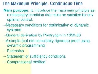
The Maximum Principle: Continuous Time. Main purpose : to introduce the maximum principle as a necessary condition that must be satisfied by any optimal control. --Necessary conditions for optimization of dynamic systems --General derivation by Pontryagin in 1956-60

The Maximum Principle: Continuous Time
E N D
Presentation Transcript
The Maximum Principle: Continuous Time Main purpose: to introduce the maximum principle as a necessary condition that must be satisfied by any optimal control. --Necessary conditions for optimization of dynamic systems --General derivation by Pontryagin in 1956-60 --A simple (but not completely rigorous) proof using dynamic programming -- Examples -- Statement of sufficiency conditions -- Computational method
2.1 Statement of the problem Optimal control theory deals with the problem of optimization of dynamic systems 2.1.1 The Mathematical Model State equation where state variables, x(t)En ,control variables, u(t) Em , and f : En x Em x E1 En. f is assumed to be continuously differentiable. The path x(t), t[0,T] is called a state trajectory and u(t), t[0,T] is called a control trajectory.
2.1.2 Constraints Admissible control u(t),t [0,T] is piecewise continuous and satisfies, in addition, 2.1.3 The Objective Function Objective function is defined as follows Where F: En x Em x E1 E1 and S: En x E1 E1. F and S are assumed to be continuously differentiable.
2.1.4 The Optimal Control Problem The problem is to find an admissible control u* , which maximizes the objective function (2.3) subject to (2.1) and (2.2). We restate the optimal control problem as: Control u* is called optimal control, x* is called the optimal trajectory under u*, J(u*) or J* will denote optimal value of J.
Case 1. The optimal control problem (2.4) is said to be in Bolza form. Case 2. When S0, it is said to be in Lagrange form. Case 3. When F 0, it is said to be in Mayer form, If F 0 and S is linear, it is in linear Mayer form, i.e., where c=(c1,c2,…,cn) En.
The Bolza form can be reduced to the linear Mayer form,we define a new state vector y=(y1,y2,…,yn+1), having n+1 components defined as follows:yi=xi for i=1,2…,n and so that the objective function is J=cy(T)=yn+1(T). If we now integrate (2.6) from 0 to T, we have which is the same as the objective function J in (2.4)
Statement of Bellman’s Optimality Principle “An optimal policy has the property that whatever the initial state and initial decision are, the remaining decisions must constitute an optimal policy with regard to the state resulting from the first decision.”
PRINCIPLE OF OPTIMALITY Jbe Jab b Jbce e a c Assertion: If abe is the optimal path from a to e, then be is the optimal path from b to e. Proof: Suppose it is not. Then there is another path (note that existence is assumed here) bce which is optimal from b to e, i.e. Jbce > Jbe but then Jabe = Jab+Jbe< Jab+ Jbce= Jabce This contradicts the hypothesis that abe is the optimal path from a to e.
A Dynamic Programming Example Stagecoach Problem Costs:
Solution: Let 1-u1-u2-u3-10 be the optimal path. Let fn(s,un) be the minimal cost path given that current state is s and the decision taken is un . fn*(s) = min f (s,un) = fn(s,un*) un This is the Recursion Equation of D.P. It can be solved by a backward procedure – which starts at the terminal stage and stops at the initial statge.
Note: 1-2-6-9-10 with cost=13 is a greedy path that minimizes costat eachstage. This may not be minimal cost solution, however, E.g.1-4-6 is cheaper overall than 1-2-6.
2.2 Dynamic Programming and the Maximum Principle 2.2.1 The Hamilton – Jacobi- Bellman Equation where for s t , Principle of Optimality An optimal policy has the property that, whatever the initial state and initial decision are, the remaining decision must constitute an optimal policy with regard to the outcome resulting from the first decision.
The change in the objective function consists of two parts: 1. The incremental changes in J from t to t+t, which is given by the integral of F(x,u,t) from t to t+t, 2. The value function V(x+x, t+t) at time t+t. In equation form we have Since F is continuous, the integral in (2.9) is approximately F(x,u,t) t so that we rewrite (2.9) as
Assume that V is a continuously differentiable. Use Taylor series expansion of V with respect to t and obtain • Substituting for x from (2.1) • canceling V(x,t) on both sides and then dividing by t • we get
Let t 0 with the boundary condition Vx(x,t) can be interpreted as the marginal contribution of the state variable x to the maximized objective function. Denote it by (t) En called the adjoint (row) vector i.e.,
We introduce the so-called Hamiltonian or The (2.14) can rewritten as the following (2.19) will be called the Hamilton-Jacobi-Bellman equation or, HJB equation.
From (2.19) we can get Hamiltonian maximizing condition of the maximum principle canceling the term Vt on both sides, we obtain for all u (t). Remark: Hdecouples the problem over time by means of (t), which is analogous to dual variables or shadow prices in Linear Programming.
2.2.2 Derivation of the Adjoint Equation Let where for a small positive . Fix t and use H-J-B equation (2.19) LHS=0 from (2.19) since u* maximizes [H+Vt]. RHS will be zero if u*(t) also maximizes H+Vt with x(t) as the state. In general x(t) x*(t), thus RHS 0, But then RHS|x(t)=x*(t)=0 RHS is maximized at x(t)=x*(t).
Since x(t) is unconstrained, we haveRHS/ x |x(t)=x*(t) = 0 or, By definition of H Note: (2.25) assumes V to be twice continuously differentiable.
Using (2.25) and (2.26) we have Using (2.16), we have From (2.18), we have
Terminal boundary condition or transversality condition: (2.28) and (2.29) can determine the adjoint variables. From (2.28), we can rewrite the state equation as From (2.28), (2.29), (2.30) and (2.1), we get (2.31) is called a canonical system of equation or canonical adjoints.
Free and Fixed End Point Problems S 0 (T) = 0 no salvage value x(T) fixed (T) = some constant (given)
2.2.3 The Maximum Principle The necessary conditions for u* to be an optimal control are:
2.2.4 Economic Interpretation of the Maximum Principles where F is considered to be the instantaneous profit rate measured in dollars per unit of time, and S[x,T] is the salvage value, in dollars. Multiplying (2.18) formally by dt and from (2.1), we have F(x,u,t)dt: direct contribution to J in $ from t to t+dt. dx: indirect contribution to J in dollars. Hdt: total contribution to J from time t to t+dt when x(t)=x and u(t) =u in the interval [t,t+dt].
By (2.28) and (2.29) we have Rewriting the first equation as -d: marginal cost of holding capital from t to t+dt Hxdt: marginal revenue of investing the capital Fxdt: direct marginal contribution fxdt: indirect marginal contribution Thus, adjoint equation implies MC = MR
Example 2.1 Consider the problem subject to the state equation and the control constraint Note that T=1, F=-x, S=0, and f =u. Because F=-x, we can interpret the problem as one of minimizing the (signed) area under the curve x(t) for 0t 1.
Solution.First we form the Hamiltonian and note that, because the Hamiltonian is linear in u, the form of the optimal control, i.e., the one that would maximize the Hamiltonian, is or referring to the notation in Section 1.4,
To find , we write the adjoint equation Because this equation does not involve x and u, we can easily solve it as It follows that (t) = t-1 0 for all t[0,1], and since we can set u*(1)=-1, which defines u at the single point t=1, we have the optimal control
Substituting this into the state equation(2.34) we havewhose solution is The graphs of the optimal state and adjoint trajectories appear in Figure 2.2. Note that the optimal value of the objective function is J*= -1/2.
Figure 2.2 Optimal State and Adjoint Trajectories for Example 2.1
Example 2.2 Let us solve the same problem as in example 2.1 over the interval [0,2] so that the objective is to The dynamics and constraints are (2.33) and (2.34), respectively, as before. Here we want to minimize the signed area between the horizontal axis and the trajectory of x(t) for 0t2.
Solution.As before the Hamiltonian is defined by (2.36) and the optimal control is as in (2.38). The adjoint equation is the same as (2.39) except that now T=2 instead of T=1. The solution of (2.44) is easily found to be Hence the state equation (2.41) and its solution (2.42) are exactly the same. The graphs of the optimal state and adjoint trajectories appear in Figure 2.3. Note that the optimal value of the objective function here is J*=0.
Figure 2.3 Optimal State and Adjoint Trajectories for Example 2.2
Example 2.3 The next example is: subject to the same constraints as in Example 2.1, namely, Here F= - (1/2)x2 so that the interpretation of the objective function (2.46) is that we are trying to find the trajectory x(t) in order that the area under the curve (1/2)x2 is minimized.
Solution. The Hamiltonian is which is linear in u so that the optimal policy is The adjoint equation is Here the adjoint equation involves x so that we cannot solve it directly. Because the state equation (2.47) involves u, which depends on , we also cannot integrate it independently without knowing .
The way out of this dilemma is to use some intuition. Since we want to minimize the area under (1/2)x2 and since x(0)=1, it is clear that we want x to decrease as quickly as possible. Let us therefore temporaily assume that is nonpositive in the interval [0,1] so that from (2.49) we have u=-1 throughout the interval. (In Exercise 2.5, you will be asked to show that this assumption is correct.) With this assumption, we can solve (2.47) as
Substituting this into (2.50) gives Integrating both sides of this equation from t to1 gives or which, using (1)=0, yields
The reader may now verify that (t) is nonpositive in the interval [0,1], verifying our original assumption. Hence (2.51) and (2.52) satisfy the necessary conditions. In Exercise 2.6, you will be asked to show that they satisfy sufficient conditions derived in Section 2.4 as well, so that they are indeed optimal. Figure 2.4 shows the graphs of the optimal trajectories. • It would be clearly optimal if we could keep x*(t)=0, t ≥1. • This is possible by setting
Figure 2.4 Optimal Trajectories for Example 2.3 and Example 2.4
Example 2.4 Let us rework Example 2.3 with T=2, i.e, Subject to the constraints: It would be clearly optimal if we could keep x*(t)=0, t ≥1. This is possible by setting: 1 t≤1 u*(t)= -1 t ≥1. Note u*(t)=0, t≥1 is singular control.
2.4 Sufficient Conditions Since either or or both.
Theorem 2.1(Sufficiency Conditions). Let u*(t), and the corresponding x*(t) and (t) satisfy the maximum principle necessary condition (2.32) for all t[0,T]. Then, u* is an optimal control if H0(x,(t),t) is concave in x for each t and S(x,T) is concave in x.
Example 2.6: Examples 2.1 and 2.2 satisfy the sufficient conditions. Fixed-end-point problem: Transversality condition is:
2.5 Solving a TPBVP by Using Spreadsheet Software Example 2.7 Consider the problem: