discret filter implementation
discrete filter implementation for FIR and IIR filters, quantization , limit cycle

discret filter implementation
E N D
Presentation Transcript
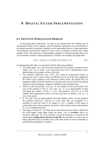
8 DIGITAL FILTER IMPLEMENTATION 8.1 THE FINITE WORD LENGTH PROBLEM In discussing filter realizations, we have so far assumed that all variables can be represented exactly in the computer, and all arithmetic operations can be performed to an infinite precision. In practice, numbers can be represented only to a finite precission. And arithmetic operations are subjects to errors, since a computer word has only a finite number of bits. The operation of representing a number to a fixed precission (that is, by a fixed number of bits) is called quantization. Consider, for example, the digital filter ( ) y n ( ) ( 1 ) ( ) ( ) 0 x n ( ) ( 1 ) = − − + + −1 (8.1) a y n 1 b b x n In implementing this filter, we must deal with the following problems: 1. The input signal ( ) x n may have been obtained by converting a continuous-time signal ( ) x t . As we know, A/D conversion gives rise to quantization errors, determining by the number of bits of the A/D. 2. The constant coefficients , general, the error in each of these coefficients can be up to the least significant bit (LSB) of the computer word. Because of these errors, the digital filter we implement differs from the desired one. Its poles and zeros are not in the desired locations, and its frequency response is different from the desired one. 3. When we form the product sum of the numbers of bits in increasing the number of bits of number. Such quantization leads to an error each time we update every time point). 4. If ( ) x n and are represented by the same number of bits, we must quantize the products , possible to avoid this error if we assign to greater than that of these products. In practice, this usually means representation of in double precision. ( ) 5. The range of values of that can be represented in fixed point is limited by the word length. Large input values can cause exceed its full scale. To avoid overflow, it may be necessary to scale down the input signal. Scaling always involves trade-off: On one hand we want to use as many significant bits as possible, but on the other hand we want to eliminate or minimize the possibility to overflow. ( ) 1 ( ) 0 ( ) 1 , cannot be represented exactly, in a b b ( ) ( 1 a ) y n− ( ) 1 , the number of bits in the result is the and . It is unreasonable to keep , and quantize ( y n a 1 ( ) y n− 1 ) ( ) ( 1 ) y n− to this (i.e., at a 1 ( ) y n ( ) y n b ( ) 0 ( ) x n ( ) ( 1 ) x n− every time they are computed. It is a number of bits equal or ( ) y n b 1 ( ) y n y n ( ) y n to overflow, that is, to 1 DIGITAL FILTERS – LESSONS (2004)
DIGITAL FILTER IMPLEMENTATION ( ) y n 6. If the output signal to be further quantized, to match the number of bits in the D/A. Such quantization is another source of error. In the remaining sections of this chapter we shall study these problems, analyze their effects, and learn how they can be solved or at least mitigated. is to be fed to the D/A converter, it sometimes needs 8.2 COEFFICIENT QUANTIZATION IN DIGITAL FILTERS When a digital filter is designed using high-level software, the coefficients of the designed filter are computed to high accuracy. MATLAB, for example, gives the coefficients to 15 decimal digits. With such accuracy, the specifications are usually met exactly (even exceeded in some bands, because the order of the filter is typically rounded upward). When the filter is to be implemented, there is usually a need to quantize the coefficients to the word length used for the implementation (whether in software or in hardware). Coefficient quantization changes the transfer function and, consequently, the frequency response of the filter. As a result, the implemented filter may fail to meet the specifications. This was a difficult problem in the past, when computers had relatively short word lengths. Today, many microprocessors designed for DSP applications have word lengths from 16 bits (about 4 decimal digits) and up to 24 in some (about 7 decimal digits). In the future, even longer words are likely to be in use, and floating-point arithmetic may become commonplace in DSP applications. However, there are still many cases in which finite word length is a problem to be dealt with, whether because of hardware limitations, tight specifications of the filter in question, or both. We therefore devote this section to the study of coefficient quantization effects. We first consider the effect of quantization on the poles and the zeros of the filter, and then its effect on the frequency response. 8.2.1 QUANTIZATION EFFECTS ON POLES AND ZEROS { } ( ) a k ( ) ,b k ( ) b k . The Coefficient quantization causes a replacement of the exact param ters of the transfer function by corresponding approximate values difference between the exact and approximate values of each parameter can be up to the LSB of the computer, multiplied by the full-scale value of the parameter. For example, consider a second-order IIR filter e { , } ( ) ˆ ˆ a k ( ) 0 1 + ( ) 1 1 ( ) 2 2 − − + + 1 2 b b z b z ( ) = (8.2) H z ( ) ( ) − − + 1 2 a z a z ( ) 1 < 2 and a Since we are dealing only with stable filters, we know that necessarily ( ) 2 a <1. Suppose we represent each coefficient by B bits, including sign. Then, assuming we scale a so that the largest representable number is ± , the LSB for will be , and the error ( ) 1 a 2 ˆ 1 a a − 1 we scale so that the largest representable number is ± , the LSB for , and the error 2 ( ) ˆ a 1 a − 1 can be up to Replacement of the exact parameters by the quantized values causes the poles and zeros of the filter to shift their desired locations, and the frequency response to deviate from its desired shape. Usually, we are not as much interested in the deviation of the ( ) 1 2 ( ) ( ) ( ) ( ) − − − − B 2 B 1 can be up to 2 . Similarly, assuming ( ) 1 a ( ) 2 1 will be a ( ) ( ) − − − B 1 B 2 . 2 DIGITAL FILTERS – LESSONS (2004)
DIGITAL FILTER IMPLEMENTATION poles and zeros as in the deviation of the frequency response. However, it is instructive to explore the former, since this will lead to important qualitative conclusions. Consider, for example, the poles of a second-order filter, given by ( ) ( ) 1 ( ) 2 ( ) 1 2 α = − ± − ˆ a ˆ a ˆ a 0.5 0.25 (8.3) 1,2 { α } ( ) 1 , can assume only a finite number of values. Of particular interest are the ( ) 2 2B ˆ a ˆ a Since poles possible locations of complex stable poles. These are depicted by the dots in Figure 1, in the case . can assume only a finite number of values each (equal to ), the 1,2 B = 5 ????? ????? Figure 1 Possible locations of complex stable poles of second-order digital filter in direct realization, number of bits B = 5 As we see from Figure 1, the permissible locations of complex poles of the quantized filter are not distributed uniformly inside the unit circle. In particular, small values of the imaginary part are virtually excluded. The low density of permissible pole locations in the vicinity of and high-pass filters must have complex poles in the neighborhood of conclude that high coefficient accuracy is needed to accurately place the poles of such filters. Another conclusion is that high sampling rates are undesirable from the point of view of sensitivity of the filter to coefficient quantization. A high sampling rate means that the frequency response in the domain is pushed toward the low-frequency band, correspondingly, the poles are pushed toward the word length necessary for accurate representation of the coefficients. There is another realization of second –order section called coupled realization shown in Figure 2. z = z = − 1 1 is especially troublesome. Narrow-band, z = − 1 . We therefore ω z = 1 and, as we have seen, this increases 3 DIGITAL FILTERS – LESSONS (2004)
DIGITAL FILTER IMPLEMENTATION ? ?? ?????? ? ???? ???? ???? ? ? ? ? ?? ? ? ?????? ? ? ? ? ? ???? Figure 2 A coupled second-order section for cascade realization i α α The parameters second-order section that is , are the real and imaginary parts of the complex pole of the r ( ) α 2 α α α α = + = 2 r 2 i Re , (8.4) r ( ) n ( ) 1 ( ) ( ) 2 1s n , obtain the right numerator of transfer function (8.2) (for b parametrized directly in the terms of complex pole. Therefore, if each of these two parameters is quantized to the range ( , the permissible pole locations will be distributed uniformly in the unit circle. This is illustrated in Figure 3 for pole locations near is higher in this case. 1 z = ± are state-space variables and are coefficients necessary to ). This realization is ( ) 0 = , the real and imaginary parts of the , 2s c c 1 { } α α , r i 2B levels in ) − 1 1, = . As we see, the density of permissible B 5 ????? ????? Figure 3 Possible locations of complex stable poles of a second-order digital filter in coupled form, number of bits B = 5 The sensitivity of the poles of a digital IIR filter to denominator coefficient quantization usually increases with the filter order. The effect of quantization of the numerator coefficients may seems, at first glance, to be the same as that of the denominator coefficients. This, however, is not the case. As 4 DIGITAL FILTERS – LESSONS (2004)
DIGITAL FILTER IMPLEMENTATION we know, the zeros of an analog filter of the four common classes (Butterworth, Chebyshev-I, Chebyshev-II, elliptic) are always on the imaginary axis. Consequently, the zeros of a digital IIR filter obtained from an analog filter by a bilinear transform are always on the unit circle. Thus, the numerator of a second-order IIR filter has either real zeros at or a conjugate complex pair at 1 z = ± coefficients are trivial (± or ± ), so the problem of co arise. In the latter case, the numerator has the form constant gain), so only the coefficient 2cos ξ is subject to quantization. When this coefficient undergoes a small perturbation, the zeros will shift but will stay on the unit circle. The effect of such a shift on the behavior of the filter is usually minor. ξ ± = j z e effi 1 2 ( . In the former case, the cient quantization does not + ( ) cos z z ξ 1 2 ) − − − 1 2 (up to a ( ) 8.2.2 QUANTIZATION EFFECTS ON THE FREQUENCY RESPONSE Next we examine the sensitivity of the magnitude of the filter’s frequency response to coefficient quantization. We assume that { ,1 k K ≤ ≤ { , 0 i N ≤ ≤ ( ) , , e i f i ( ) , ,1 g i h i i N ≤ ≤ . For all IIR filter realizations, realization of a linear phase FIR filter, the parameters are Let us assume that the perturbations in the parameters resulting from quantization are small, and approximate the perturbation in the magnitude response first-order Taylor series: H jω) ( depends on a set of real parameters . In case of a direct realization, the parameters are { , in case of a parallel } 1 i N , in case of a cascade realization, they are b } } } ≤ ≤ and and and kx ib ia are ,1 i c N } ( ) 0 ( ) 0 } . ( H jω by a realization, they { { ( ) ( ) ≤ ≤ = { + . In case of a direct 0.5 i N ≤ ≤ K 2 ( ) N 1 h i , 0 ) ( x )( ω ∂ H j ∂ K ∑ ( ) ( ) ) ˆ ω ω − ≈ − ˆ x (8.5) H j H j x k k = k 1 k The partial derivatives on the right side of (8.5) are given by ( x ) ( x ) ∂ ω H j ∂ ∂ ω H j ∂ ( ) φ ω − j = Re e (8.6) k k where ( ) be used for estimating the effect of coefficient quantization on the magnitude response in the following manner. Let k X denote the full scale used for the coefficient must be at least as large as be half the quantization level relative to full scale, so Q length in bits). Then we have φ ω is the phase response of the filter. The approximate error formula (8.5) can kx . X k kx , and is often larger, for reasons explained below. Let Q − = B 2 (where B is the word − ≤ ˆk x Q (8.7) x X k k Substitution in (8.5) leads to the approximate inequality ( x ) ∂ ω H j ∂ K ∑ ( ) ( ) ˆ − ≤ ω ω H j H j Q x (8.8) k = k 1 k The function 5 DIGITAL FILTERS – LESSONS (2004)
DIGITAL FILTER IMPLEMENTATION ( x ) ∂ ω H j ∂ K ∑ ( ) ω = S x (8.9) k = k 1 k is the sensitivity bound of the filter. As we see, the sensitivity bound depends on the realization. The realization determines the coefficients the partial derivatives of the magnitude response with respect to the coefficients. In summary, the error in the magnitude response at any given frequency is approximately bounded by kx , their full-scale values, and ( ) ( ) ( ) ω ˆ − − ≤ ω ω B H j H j 2 S (8.10) A common way of choosing the full-scale values numerator and denominator polynomials of a direct realization, we find the coefficient having the largest magnitude and use it as the full-scale value for all the coefficients of the polynomial in question. The corresponding formulas are X is as follows. For each of the k ( ),0 ( ) MAX abs b i = ≤ ≤ X i N (8.11) num ( ),1 ( ) MAX abs a i = ≤ ≤ X i N (8.12) den ± This way, the coefficient of largest magnitude in each polynomial is represented by For parallel and cascade realizations, we scale each section separately in the same way. Another way of choosing the full-scale values is to round the largest magnitude coefficient of each polynomial upward to the nearest integer power of 2 and take the rounded value as the full scale of all the coefficients of the polynomial. The corresponding formulas are 1 . ( ) ( ) ( ) MAX abs b i i N ≤ ≤ log , 0 = 2 (8.13) X 2 num ( ) ( ) ( ) MAX abs a i i N ≤ ≤ log ,1 = 2 (8.14) X 2 den This method yields larger convenient, since the scaled coefficients are related to the true ones by simple shifts. The sensitivity bound is useful for determining a suitable word length for implementing a given filter in a given realization. Let all pass bands of the filter, and reasonable to require that the maximum deviation from the tolerance caused by quantization be no more than 10 percent of the tolerance itself (a different percentage can be chosen, depending on the application). With this requirement, (8.10) leads to X and X than the ones in (8.11) and (8.12), but is more num den δ be the minimum tolerance of p s δ the minimum tolerance of all stop bands. It is { } ( ) ω ω max S : in a pass band 0.1 δ ≥ B log (8.15) 2 p 6 DIGITAL FILTERS – LESSONS (2004)
DIGITAL FILTER IMPLEMENTATION { } ( ) ω ω max S : in a stop band 0.1 δ ≥ B log (8.16) 2 s Therefore, choosing B according to the greater of the two right sides in (8.15) and (8.16) guarantees that the error in the magnitude response resulting from quantization will deviate only slightly (if at all) from the permitted bounds in all frequency bands. Matlab functions in the Appendix compute the sensitivity bounds for the standard realizations. The procedure sensiir is for IIR filters in direct, parallel, and cascade realizations, whereas sensfir is for linear-phase FIR filters in a direct realization. Each of the two procedures returns the individual sensitivities dHmag, and the sensitivity bound S in the vector S. These are computed at frequency points, in the interval specified by the input variable theta. The procedure dhdirect, dhparal, dhcascad return the partial derivatives ∂ respective IIR realizations, and the full-scale values scale values are computed by scale2 according to (8.13) and (8.14). ( ) / ∂ ∂ ω H j x in the matrix k ( ) ω K ( ) H jω ∂ of the / kx X of the coefficients. The full- k 8.3 SCALING IN FIXED-POINT ARITHMETIC When implementing a digital filter in fixed-point arithmetic, it is necessary to scale the input and output signals, as well as certain inner signals, to avoid signals values that exceed the maximum representable number. A problem of similar nature arises in active analog filters. There, it is required to limit the signals to voltages below the saturation levels of the operational amplifiers. However, there is an important difference between the analog and the digital cases: When an analog signal exceeds its permitted value, its magnitude is limited but its polarity is preserved. When a digital signal exceeds its value, we call it an overflow. An overflow in two’s-complement arithmetic leads to polarity reversal. A number slightly larger than 1 changes to a number slightly larger than –1. Therefore, overflows in digital filter are potentially more harmful than in analog filters, and care is necessary to prohibit them, or to treat them properly when they occur. The scaling problem can be started in mathematical terms as follows. Suppose we wish to prevent the magnitude of the output signal input and output are related through a convolution ( ) y n upper limit y . Since the max ( ) { y n }( ) = x h ∗ (8.17) n we may be able to achieve this goal by properly limiting the input signal ( ) however may be undesirable because limiting is a nonlinear operation that distorts the signal. A more attractive solution is to scale the impulse response by a proportionality factor , chosen in a way that will prevent the magnitude of c exceeding the maximum value . Such a proportionality factor may also be useful in the opposite case. If the dynamic range of x n magnitude than , we can adjust to increase the range of either case, the transfer function is called a scaled transfer function. Our task is to find a scale factor that will cause possible without exceeding in magnitude. Judicious choice of a scale factor requires knowledge of certain parameters of the input signal. Accordingly, there exist x n . This, { }( ) h ∗ from c x n y max ( ) ( ) y n is such that is much smaller in as needed. In ( ) y n y c max ( ) z cH ( ) to have as large dynamic range as c y n y max 7 DIGITAL FILTERS – LESSONS (2004)
DIGITAL FILTER IMPLEMENTATION several scaling methods, differing in their assumptions on the nature and properties of the input signal. The scaling problem is obviated if floating-point arithmetic is used. However, fixed- point implementations of digital are very common, so familiarity with scaling methods and the effect of scaling on the properties of the filter is expedient. 8.3.1 TIME-DOMAIN SCALING Consider a linear, time invariant filter whose impulse response and transfer function and , respectively. Assume that the input signal ( ) h n H z bounded in magnitude by max x , and the output signal is required to be bounded in magnitude by . Both values are relative to the maximum value representable by the computer, usually taken as 1. The output signal is related to the input by the convolution formula ( ) ( ) x n is known to be are y max ∞ =∑ ( ) y n ( ) ( h m x n m ) − (8.18) = m 0 Therefore, ∞ ∞ ∑ ∑ ( ) y n ( ) h m ( ) ( ) h m ≤ ⋅ − ≤ = (8.19) x n m max x max x h 1 = = m 0 m 0 where ∞ =∑ ( ) m (8.20) h h 1 = m 0 ( ) Stability of the filter h n implies that ( ) max y n y ≤ will be achieved if we use a scale factor 1 is finite. As we see, the requirement h y = max (8.21) c max x h 1 In practice, it may be convenient to round c downward to an integer power of 2, since this facilitates scaling by bit shifting. Example 1 Suppose that an analog signal is sampled by a 12-bit A/D converter, then fed to a 16-bit filter whose transfer function is 1 ( ) = H z z− 1 0.98 − 1 If we place the sampled signal ( ) extension), the corresponding x signal to . We have max 1 y = in the lower bits of computer word (with sign x n will be 1/1 . Suppose we wish to scale the output 6 max 8 DIGITAL FILTERS – LESSONS (2004)
DIGITAL FILTER IMPLEMENTATION ∞ 1 ∑ = = = m h 0.98 50 1 0.98 − 1 = m 0 = = Therefore, the maximum scale factor is c downward to a power of 2, we get a scale factor of 0.25. Such scaling is equivalent to shifting ( ) x n by 2 bits to the right, thus losing 2 out of the 12 available bits. The lesson from this example is that scaling using c as in (8.21) potentially involves loss of accuracy of the input signal. in this case. Rounding 16/50 0.32 8.3.2 FREQUENCY-DOMAIN SCALING The scale factor given in (8.21) is often over-conservative in its use of the dynamic range of the computer word. By this we mean that the values assumed by the output signal are usually small in magnitude compared with the full scale. Less conservative scaling is provided by frequency-domain bounds, as follows. 1-norm bound: We have, by the inverse Fourier transform formula, π ∫ 1 π− ( ) y n ( ) ( ) i n ω = ω ω ω H j X j e d (8.22) 2 π Therefore, π ∫ 1 π− ( ) y n ( ) ( ) ≤ ω ⋅ ω ω H j X j d (8.23) 2 π Define π ∫ 1 π ( ) ( ) = ω = ω ω X max ω X j , H H j d (8.24) ∞ 1 2 π − ( ) X jω , and the quantity The quantity X called 1-norm of the scale factor ∞ is called the infinity norm of . If ( X 1 is H H jω) ( ) y n ≤ ∞ is finite, we can guarantee that by using y max y = max c (8.25) H X ∞ 1 Infinity-norm bound: By reversing the roles of H and X in (8.25), we get the scale factor y = max c (8.26) H X ∞ 1 This scale factor is applicable in case particularly useful when the input signal is narrow band. For example, if ( ) X , the 1-norm of the input signal, is finite. It is 1 x n is known 9 DIGITAL FILTERS – LESSONS (2004)
DIGITAL FILTER IMPLEMENTATION to be sinusoidal, the scale factor (8.26) guarantees that the amplitude of the sinusoid at the output of the filter not exceed . max y 2-norm bound: Unlike the preceding bounds, the bound we introduce now is probabilistic. Define π 1 π−∫ ( ) 2 = ω dω H H j (8.27) 2 2 π Note that (8.27) is identical to the square root of the noise gain of the filter. Let us assume that the input ( ) x n is a wide-sense stationary signal having power spectral density . Then, we can bound the variance of the output signal as follows: ( x K jω) π ∫ π ∫ 1 π 1 π ( ) ( ) ( ) 2 2 γ = j ω ω = j ω ω ≤ K d K H j K H (8.28) y y x x ∞ 2 2 2 π − π − Therefore, if we know the maximum possible value of the power spectral density of the input signal, and we require that the variance of the output signal not exceed get the scale factor γ , we y ,max γ y ,max K c = (8.29) 2 H x ∞ 2 ( ) y n γ ( ) y n Bounding the variance of why we refer to (8.29) as probabilistic scaling. If, for example, we take the probability of ( ) y n exceeding The four norms we have introduced are known to satisfy the relationship does not guarantee boundedness of , and this is 0.1y ≈ 2 max , y ,ma x 1. y is expected to be low ma x ≤ ≤ ≤ 1 (8.30) H H H h ∞ 1 2 This, however, does not imply that since the different scaling rules also depend on K nature of the input signal and its bounds. 1 always provides the best (largest) scale factor, x , , max y γ H , X ∞, X and max y ,max 1 ∞. Therefore, judicious choice of scaling method requires knowledge about the x 8.3.3 MATLAB IMPLEMENTATION OF FILTER NORMS Exact computation of norms we have presented is not possible in general for rational filters (with the exception of used instead. High accuracy is not required, since the scale factor resulting from those norms is usually Appendix implements the computation of the four filter norms. The time-domain norm h is computed by calling the function filter with a unit-sample input, and adding 2). However, numerical approximations can be H 2 rounded to an integer power of 2. The procedure filnorm in the 1 1 For example, if ( ) 2 For some realizations scaling factors can be absorbed into the filter coefficients. In this case the scaling factors need not to be limited to an integer power of 2. y n has Gaussian probability density, this probability is about 0.0016. 10 DIGITAL FILTERS – LESSONS (2004)
DIGITAL FILTER IMPLEMENTATION terms ( ) is computed by calling nsgain and taking the square root of the result. The norm H is approximated by the maximum of the magnitude response, computed on a dense grid. Finally, the norm grid and approximating the integral by Simpson’s rule. h n until the relative error drops below a prescribed threshold. The norm H 2 ∞ 1 is computed by evaluating the magnitude response on a dense H 8.3.4 SCALING OF INNER SIGNALS Our discussion so far has concentrated on input scaling of a transfer function to avoid overflow of the output. In realizing a filter, inner (or intermediate) signals are always present, so we need to concern ourselves with potential overflow problems in such signals as well. There are four types of inner signal: 1. A signal resulting from delaying another signal. Such a signal can never overflow if the signal at the input of the delay does not. 2. A signal resulting from multiplying a signal by a constant. Assuming that both factors in the product are scaled below 1, the product is also less than 1 in magnitude, so it cannot overflow. 3. A signal resulting from adding two signals to form a partial sum, which is later used as an operand in another sum. We assume that such a signal is not used for any other purpose in the filter or outside it. Addition of two signals can potentially lead to overflow. However, two’s-complement arithmetic has the following important property: If a sum of numbers ( overflows in partial sums cancel out and do not affect the signal result. For example, suppose that 1 2 3 x x x + + does not overflow, and the computation is performed in the in the order ( 1 2 x x + the overflow is ignored, the final result will still be correct. The reason is that two’s-complement is a special case of modular arithmetic (i.e., a number represented by ( , assuming that the binary point is immediately to the right of the sign bit), hence standard rules of modular addition apply to it. The conclusion is that, if the filter is implemented in two’s-complement arithmetic, overflows in partial sums can be ignored. 4. A signal resulting from adding two signals to form a final sum, which is needed elsewhere in the filter or outside it. Such signal must be scaled similarly to the output signal, since its overflow is potentially harmful. This is done by computing the transfer function from the input to the signal in question and using one of the scaling methods described earlier. It is also recommended, in most applications, to detect overflows of such signals and replace the overflowed signal by the corresponding saturation value. For example, if it is detected that 1 ≥ , x should be replaced by 1 2 , 1 x < − x should be replaced by saturation mode, in which this operation is performed automatically after the addition. n > ) does not overflow, 2 n ) + + . Then, even if overflows and x x x 3 1 2 is x ) 2 x mod ( ) − − B 1 − ; if it is detected that x − 1 . Most DSP microprocessors have a Example 2 In the direct realization shown in Figure 4 (chapter 7) there are 15 inner signals, in addition to the output signal. However, only the signals u n and fourth type. The former because it is used more than once inside the filter, and the latter because it is used outside it. The transfer function from ( ) ( ) y n are of the ( x n to u n is ) ( ) 11 DIGITAL FILTERS – LESSONS (2004)
DIGITAL FILTER IMPLEMENTATION ( ) ( ) U z X z 1 = ( ) A z so one of the scaling methods explained previously should be used for it. In the transposed direct realization shown in Figure 7 (chapter 7), only the output signal is of the fourth type. Any overflow generated at one of the adders along the central lane will propagate through the delays and will eventually reach However, if the input is properly scaled to avoid overflow in realization will be insensitive to intermediate overflows. In this respect, the transposed direct realization offers an advantage over the direct realization. ( ) y n ( ) y n . ( ) y n , the entire 8.3.5 SCALING IN PARALLEL AND CASCADE REALIZATION We now discuss in detail scaling procedures for parallel and cascade realizations for IIR filters. As we saw in the last example, the transposed direct realization has an advantage over the direct realization, in that there is no need to scale inner signals. We therefore consider only parallel and cascade realizations in which the second-order sections are in a transposed direct realization3. Figure 4 illustrates a parallel connection of three second-order sections (delays are representable by factors , and summing junctions by open circles). The scaling procedure is as follows: 1. The input coefficients , the output signal of the section. As we have explained, this scaling depends on the assumptions made on the input signal, and on the norm used. The same scale factor should be applied to both coefficients of a specified section, but different factors are permitted at different sections. The Figure 4 are assumed to be scaled already. 2. The coefficients λ are computed to make total gains of all sections (including the branch of constant gain ) equal to the corresponding gains in the unscaled transfer function, up to a common proportionality factor. For example, if where scaled down by 2 compared with by 2. 3. The dynamic range of is checked using the scaled transfer function. If it is found that can overflow, all prevent (or decrease the probability of) this overflow. If it is found that the dynamic range of is small relative to full scale, all by a common factor. 4. In the preceding steps, all factors are usually taken as integer powers of 2. This way, factors greater than 1 can be implemented by left shifts, and factors smaller than 1 can be implemented by right shifts. z− 1 mf at each section are scaled to prevent overflow of ( ) n kv mf shown in k 0c 1f , 2f 2 λ 1λ 3f , 4f , then must be larger than ( ) y n ( ) y n k λ must be decreased by a common factor, to ( ) k λ may be increased y n Example 3 Consider parallel realization of IIR filter with coefficients quantized to 16 bits with 3 For some hardware implementations it make sense to use other structures. E.g. standard DSP architectures are typically more suitable for noncanonical realization. This will be demonstrated in the last exercise “Hardware Implementation of Digital Filters”. 12 DIGITAL FILTERS – LESSONS (2004)
DIGITAL FILTER IMPLEMENTATION − − − × × − × 20 20 1 8909 2 1 30365 2 28813 2 13038 2 + 22869 2 15710 2 19504 2 1 25279 2 − z ( ) − = − × + + 17 H z 24984 2 − − − − − + × 14 1 14 2 z z − − − − − × × + × × × 17 17 1 16 30199 2 1 28072 2 − z + + − − − − − − × 14 1 14 2 15 1 z z z = Suppose we know that the input signal satisfies scaling such that the variance of the signal at the output of each section, as well as at the output of the complete filter, will not exceed 0.1. This implies that the 2-norm fo each section must be no larger than 1 after scaling. The 2-norms of the tree unscaled sections are computed by the program filnorm and found to be 0.1528, 0.3805, and 0.4677. Therefore, the first section can be scaled by 4, the second by 2, and the third by 2. This is done by doubling the numerator coefficients of the second and the third sections, and quadrupling the numerator coefficients of the first. The 2-norm of complete filter is 0.3248, so the transfer function can be scaled by 2 to increase the dynamic range. We therefore complete the scaling procedure taking . We decide to use 2-norm K 0.1 x ∞ λ = λ = λ = λ = 2, 0.5, 1 (8.31) 0 1 2 3 ???? ???? ? ??? ????? ?? ? ? ? ??? ?? ??? ?? ? ??? ?? ??? ?? ? ? ? ?? ? ?? ??? ?? ? ??? ?? ??? ?? ? ? ? ?? ? ?? ??? ?? ? ??? Figure 4 Scaling for a parallel realization (second-order sections in a transposed direct realization). 13 DIGITAL FILTERS – LESSONS (2004)
DIGITAL FILTER IMPLEMENTATION We now turn our attention to scaling of cascade realizations. Unlike a parallel realization, here we must choose the order of the sections in the cascade, since scaling depends on this order. There is no simple rule for choosing the best order in cascade realization: It depends on the nature of the input signal, the norm used for scaling, and the specified filter. Ordering rules have been proposed in the literature but are not discussed here. We use the order provided by the program pairz. We reiterate that this program orders the complex poles in decreasing order of closeness to the unit circle (i.e., the poles closest to the unit circle appear first, and so on). Figure 5 illustrates a cascade connection of three second-order sections. Let denote the second-order sections from left to right (not including the scale factors). The scaling procedure is as follows. For each k , starting from 1 and continuing until all sections are exhausted, choose to avoid overflow in the transfer function ( ) z H k k λ k =∏ ( ) z λ H i i i 1 At the kth stage, the factors { is free to choose. After this procedure has been completed, the output of overflow, but the total gain will be stage is therefore to decrease one of the times an integer power of 2. This way, the input-output transfer function will be the desired scaled by a power of 2, as in the case of parallel realization. ( ) H z } k λ λ ≤ ≤ − have already been determined, so only ,1 i k 1 i ( ) y n will be free . The final ) ∏ k λ (0 k λ instead desired value b such that ∏ k ( ) 0 k λ will be equal to b k Example 4 We look again at the IIR filter discussed in Example 3. The cascade decomposition of the filter, with coefficients quantized to 16 bits, is − − − − × + 14 1 2 1 28587 2 1 30365 2 z z − × z z × ( ) − = × ⋅ 20 H z 29414 2 − − − − − × + 14 1 14 2 z 15710 2 1 1 25279 2 − z − − − − − × + + 14 1 2 1 1 30493 2 1 28072 2 − z × ⋅ ⋅ − − − − − × + 14 1 14 2 15 1 z 13038 2 z z = Assume, as in Example 3, that the input signal satisfies 2-norm scaling such that the variance of the signal at the output of each section will not exceed 0.1. The program filnorm gives the following 2-norms: . We decide to use K 0.1 x ∞ = = = H 1.8958, H H 1.8730, H H H 11.5802 1 1 2 1 2 3 2 2 2 λ = λ = ( ) 0 λ λ = From the first value we get that third that the to account for b ( 0.8976 × ≈ ) 0 2b , from the second that and . We decide to decrease . This gives an overall gain of , quantized to 16 bits. In summary, , and from the 0.5 0.5 1 1 2 − − λ λ λ = λ = 4 3 2 . Therefore, 2 . Finally, we must decrease one of 2 λ 19 2− × 29414 1 1 2 3 2 3 k λ from 1 to , which is equal to ) − 15 29414 2 ( − − λ = λ = × λ = 15 3 0.5, 29414 2 , 2 1 2 3 14 DIGITAL FILTERS – LESSONS (2004)
DIGITAL FILTER IMPLEMENTATION ? ? ? ? ? ? ? ? ? ? ? ? ???? ???? ?? ?? ??? ? ? ?? ??? ?? ??? ?? ??? ?? ?? ?? ? ? ? ?? ??? ?? ??? ?? ??? Figure 5 Scaling for a cascade realization (second-order sections in a transposed direct realization). 8.4 ZERO-INPUT LIMIT CYCLES IN DIGITAL FILTERS When a stable linear filter receives no input, and its internal state has nonzero initial conditions, its output decays to zero asymptotically. This follows because the response of each pole of the filter to initial conditions is a geometric series with parameter less than 1 in magnitude. However, the analysis that leads to this conclusion is based on the assumption that signals in the filter are represented to infinite precision, so they obey mathematical formulas exactly. Quantization resulting from finite word length is a nonlinear operation, so stability properties of linear systems do not necessary hold for a filter subject to quantization. Indeed, digital filters can exhibit sustained oscillations when implemented with finite word length. Oscillations resulting from nonlinearities are called limit cycles. Limit cycle phenomena are different from the noiselike behavior caused by quantization. Quantization effects are noiselike when the signal level is large and relatively fast varying, rendering the quantization error at any given time nearly independent of the errors at the past times. When the signal level is low, errors caused by quantization become correlated. When the input signal is zero, randomness disappears, and the error behavior becomes completely deterministic. Oscilations in the absence of input are called zero-input limit cycles. Such oscillations are periodic, but not necessarily sinusoidal. They are likely to appear whenever there is feedback in the filter. Digital IIR filters always have inner feedback paths, so they are susceptible to limit cycle oscillations. On the other hand, FIR filters are feedback free, so they are immune to limit cycles. This is yet another advantage of FIR filters over IIR filters. Limit cycles may be troublesome in applications such as speech and music, because resulting signal may be audible. Mathematical analysis of limit cycles is difficult except for first-order filters. We shall therefore omit most mathematical details, and restrict our discussion to some examples. Example 5 Consider the first-order filter ( ) y n ( ) ( ) x n = − − + 0.625 y n 1 Suppose that we implement the filter with 4-bit rounding arithmetic, so the least significant bit is 1/8. Let the input signal ( ) x n be zero and ( ) 0 = . Then y 3/ 8 15 DIGITAL FILTERS – LESSONS (2004)
DIGITAL FILTER IMPLEMENTATION ( ) 1 ( ) 1 = − ( ) 2 = − = − 5/64 = , and this will be rounded to ( ) 2 1/ y = ( ) 4 5/6 y = ( ) 1/ y n = . Next , and this will be rounded to ( ) 4 y = 1/8 ( )= − ω π = , and this y 15/6 4 y 1/ 4 y 5/3 2 ( ) 3 will be rounded to . Next , and this will be rounded to for all even n 8 8 4 y ( ) 3 = − . Next . From this n y 1/8 1/8 point on we will have get a constant amplitude oscillation whose frequency is 1/8. and for all odd and whose amplitude is . We y n o Example 6 Next consider the same filter, but implemented with 4-bit truncation arithmetic. The sequence of values of the output signal will now be ( ) y n = − /8, 1/8, 0, 0 − ,… 3 /8, 1 /4,1 ( ) 4 As we see, truncation of there is no limit cycle. makes it zero, thus stopping the oscillations. This time y Example 7 Consider the filter y n ( ) ( ) ( ) x n = − + 0.625 y n 1 with 4-bit rounding arithmetic. This time the output sequence is ( ) y n = … 3/8,1 /4, 1/8,1/8,1/8, As we see, the output reaches a constant nonzero value. This phenomenon is called zero-frequency limit cycle. Example 8 For the same filter as in Example 7, but with truncation arithmetic and the same initial condition, will reach zero as in Example 6. ) ( y n Example 9 Consider the filter from Example 7, but with truncation arithmetic and initial condition . Then ( ) 0 = − y 3/8 ( ) y n = − 8, 1/ − − 1/8, 1/8, − − 1/8,… 3 / 4, We get zero-frequency limit cycle again, this time with a negative constant value. The lesson from this example is that the existence and nature of limit cycles in first- order filters depend on the filter in question, the quantization level, the method of quantization, and the initial conditions. Limit cycles in second-order filters are much more difficult to analyze. As in the case of first-order filters, limit cycles are possible at both frequencies 0 and . However, second-order filters can also sustain limit cycles at other frequencies. The frequency and amplitude of the limit cycle (if it exists) depend on the coefficients, initial conditions, quantization method, and word length. However, in case of a second-order section they also depend on the realization. In particular, the coupled realization presented on Figure 2 is less susceptible to limit cycles than a direct π 16 DIGITAL FILTERS – LESSONS (2004)
DIGITAL FILTER IMPLEMENTATION realization. The coupled realization is presented by the state-space equations. It is possible to show that the coupled realization can be made completely free of zero-input limit cycles if two precautions are taken in its implementation: 1. Magnitude truncation, also called rounding toward zero, is used instead of rounding or truncation. The magnitude truncation of a number is the number ( ) a sign a . This method is seldom implemented in hardware, so it usually requires special programming. 2. Magnitude truncation of each component of state s both product (by coefficients and double precission. a ( n+ ) is performed after 1 i α α ) are formed and added (subtracted) in r 17 DIGITAL FILTERS – LESSONS (2004)
DIGITAL FILTER IMPLEMENTATION APPENDIX - MATLAB PROGRAMS function [dHmag,S] = sensiir(typ,b,a,K,theta); % Synopsis: [dHmag,S] = sensiir(typ,b,a,K,theta). % Computes the sensitivity bound for the magnitude response of % an IIR filter to coefficient quantization. % Input parameters: % typ: 'd' for direct realization % 'p' for parallel realization % 'c' for cascade realization % b, a: numerator and denominator polynomials % K: number of frequency points % theta: frequency interval (2-element vector). % Output parameters: % dHmag: the partial derivative matrix, M by K, where M is the % number of coefficients in the realization % S: the sensitivity bound, 1 by K. Hangle = exp(-j*angle(frqresp(b,a,K,theta))); if (typ == 'd'), [dH,sc] = dhdirect(b,a,K,theta); elseif (typ == 'p'), [c,nsec,dsec] = tf2rpf(b,a); [dH,sc] = dhparal(nsec,dsec,c,K,theta); elseif (typ == 'c'), c = b(1); v = roots(a); u = roots(b); [nsec,dsec] = pairpz(v,u); [dH,sc] = dhcascad(nsec,dsec,c,K,theta); end [M,junk] = size(dH); dHmag = real(dH.*(ones(M,1)*Hangle)); S = sum(abs((sc*ones(1,K)).*dHmag)); function [dH,sc] = dhdirect(b,a,K,theta); % Synopsis: [dH,sc] = dhdirect(b,a,K,theta). % Computes the derivatives of the magnitude response of an % IIR filter in direct realization with respect to the % parameters, and a scaling vector for the parameters. % Input parameters: % b, a: the numerator and denominator polynomials % K: number of frequency points % theta: frequency interval (2-element vector). % Output parameters: % dH: matrix of partial derivatives of |H(theta)| % sc: a scaling vector. % Part of software package for the book: % A Course in Digital Signal Processing % by Boaz Porat, John Wiley & Sons, 1997 dHn = []; dHd = []; scn = []; scd = []; H = frqresp(b,a,K,theta); for k = 0:length(b)-1, dHn = [dHn; frqresp([zeros(1,k),1],a,K,theta)]; end for k = 1:length(a)-1, dHd = [dHd; -frqresp([zeros(1,k),1],a,K,theta).*H]; end scn = scale2(b)*ones(length(b),1); scd = scale2(a)*ones(length(a)-1,1); dH = [dHn; dHd]; sc = [scn; scd]; end function [dH,sc] = dhparal(nsec,dsec,c,K,theta); % Synopsis: [dH,sc] = dhparal(nsec,dsec,c,K,theta). % Computes the derivatives of the magnitude response of an % IIR filter in parallel realization with respect to the 18 DIGITAL FILTERS – LESSONS (2004)
DIGITAL FILTER IMPLEMENTATION % parameters, and a scaling vector for the parameters. % Input parameters: % nsec, dsec, c: parameters of the parallel realization % K: number of frequency points % theta: frequency interval (2-element vector). % Output parameters: % dH: matrix of partial derivatives of |H(theta)| % sc: a scaling vector. dHn = []; dHd = []; scn = []; scd = []; [M,junk] = size(nsec); for k = 1:M, if (dsec(k,3) == 0), [dHt,sct] = dhdirect(nsec(k,1),dsec(k,1:2),K,theta); dHn = [dHn; dHt(1,:)]; dHd = [dHd; dHt(2,:)]; scn = [scn; sct(1)]; scd = [scd; sct(2)]; else, [dHt,sct] = dhdirect(nsec(k,:),dsec(k,:),K,theta); dHn = [dHn; dHt(1:2,:)]; dHd = [dHd; dHt(3:4,:)]; scn = [scn; sct(1)*ones(2,1)]; scd = [scd; sct(2)*ones(2,1)]; end end dH = [dHn; dHd; ones(1,K)]; sc = [scn; scd; scale2(c)]; function [dH,sc] = dhcascad(nsec,dsec,c,K,theta); % Synopsis: [dH,sc] = cascad(nsec,dsec,c,K,theta). % Computes the derivatives of the magnitude response of an % IIR filter in cascade realization with respect to the % parameters, and a scaling vector for the parameters. % Input parameters: % nsec, dsec, c: parameters of the cascade realization % K: number of frequency points % theta: frequency interval (2-element vector). % Output parameters: % dH: matrix of partial derivatives of |H(theta)| % sc: a scaling vector. dHn = []; dHd = []; scn = []; scd = []; cntd = 0; cntn = 0; [M,junk] = size(nsec); H = ones(1,K); for k = 1:M, if (nsec(k,3) ~= 0 & abs(nsec(k,2)) ~= 2), Ht = frqresp(nsec(k,:),dsec(k,:),K,theta); [dHt,sct] = dhdirect(nsec(k,:),dsec(k,:),K,theta); H = Ht.*H; dHn = [dHn; dHt(2,:)./Ht]; cntn = cntn+1; dHd = [dHd; dHt(4:5,:)./(ones(2,1)*Ht)]; cntd = cntd+2; scn = [scn; sct(2,1)]; scd = [scd; sct(4:5,1)]; end end dHn = c*(ones(cntn,1)*H).*dHn; dHd = c*(ones(cntd,1)*H).*dHd; dH = [dHn; dHd; H]; sc = [scn; scd; scale2(c)]; function s = scale2(a); % Synopsis: s = scale2(a). % Finds a power-of-2 full scale for the vector a. s = exp(log(2)*ceil(log(max(abs(a)))./log(2))); function [dHmag,S] = sensfir(h,K,theta); % Synopsis: [dHmag,S] = sensfir(h,K,theta). % Computes the sensitivity bound for the magnitude response of % a linear phase FIR filter to coefficient quantization. % Input parameters: % h: vector of coefficients % K: number of frequency points 19 DIGITAL FILTERS – LESSONS (2004)
DIGITAL FILTER IMPLEMENTATION % theta: frequency interval (2-element vector). % Output parameters: % dHmag: the partial derivative matrix, M by K, where M is the % number of coefficients in the realization % S: the sensitivity bound, 1 by K. Hangle = exp(-j*angle(frqresp(h,1,K,theta))); N = length(h) - 1; dH = []; if (sign(h(1))==sign(h(N+1))), pm = 1; else, pm = -1; end for k = 0:floor((N-1)/2), dH = [dH; frqresp( ... [zeros(1,k),1,zeros(1,N-1-2*k),pm,zeros(1,k)],1,K,theta)]; end if (rem(N,2) == 0), dH = [dH; frqresp([zeros(1,N/2),1,zeros(1,N/2)],1,K,theta)]; end sc = scale2(h); [M,junk] = size(dH); dHmag = real(dH.*(ones(M,1)*Hangle)); S = sc*sum(abs(dHmag)); function H = qfrqresp(typ,B,b,a,K,theta); % Synopsis: H = qfrqresp(typ,B,b,a,K,theta). % Computes the frequency response of a filter subject % to coefficient quantization. % Input parameters: % typ: 'd' for direct, 'p' for parallel, 'c' for cascade % b, a: numerator and denominator polynomials % K: number of frequency points % theta: frequency interval (2-element vector). % Output parameters: % H: the frequency response. if (typ == 'd'), scn = (2^(B-1))/scale2(b); b = (1/scn)*round(scn*b); scd = (2^(B-1))/scale2(a); a = (1/scd)*round(scd*a); H = frqresp(b,a,K,theta); elseif (typ == 'p'), [c,nsec,dsec] = tf2rpf(b,a); sc = (2^(B-1))/scale2(c); c = (1/sc)*round(sc*c); [M,junk] = size(nsec); H = c; for k = 1:M, nt = nsec(k,:); dt = dsec(k,:); if (dt(3) == 0), dt = dt(1:2); nt = nt(1); end scn = (2^(B-1))/scale2(nt); nt = (1/scn)*round(scn*nt); scd = (2^(B-1))/scale2(dt); dt = (1/scd)*round(scd*dt); H = H + frqresp(nt,dt,K,theta); end elseif (typ == 'c'), c = b(1); v = roots(a); u = roots(b); [nsec,dsec] = pairpz(v,u); sc = (2^(B-1))/scale2(c); c = (1/sc)*round(sc*c); [M,junk] = size(nsec); H = c; for k = 1:M, nt = nsec(k,:); dt = dsec(k,:); if (dt(3) == 0), dt = dt(1:2); nt = nt(1:2); end scn = (2^(B-1))/scale2(nt); nt = (1/scn)*round(scn*nt); scd = (2^(B-1))/scale2(dt); dt = (1/scd)*round(scd*dt); H = H.*frqresp(nt,dt,K,theta); end end function [h1,H1,H2,Hinf] = filnorm(b,a); % Synopsis: [h1,H1,H2,Hinf] = filnorm(b,a). % Computes the four norms of a rational filter. % Input parameters: % b, a: the numerator and denominator polynomials. % Output parameters: % h1: sum of absolute values of the impulse response % H1: integral of absolute value of frequency response % H2: integral of magnitude-square of frequency response 20 DIGITAL FILTERS – LESSONS (2004)
DIGITAL FILTER IMPLEMENTATION % Hinf: maximum magnitude response. [h,Z] = filter(b,a,[1,zeros(1,99)]); h1 = sum(abs(h)); n = 100; h1p = 0; while((h1-h1p)/h1 > 0.00001), [h,Z] = filter(b,a,zeros(1,n),Z); h1p = h1; h1 = h1 + sum(abs(h)); n = 2*n; end H2 = sqrt(nsgain(b,a)); N = 2 .^ ceil(log(max(length(a),length(b))-1)/log(2)); N = max(16*N,512)+1; temp = abs(frqresp(b,a,N)); Hinf = max(temp); temp = [1,kron(ones(1,(N-1)/2-1),[4,2]),4,1].*temp; H1 = sum(temp)/(3*(N-1)); LITERATURE [1] Porat, B: A Course in Digital Signal Processing. John Wiley & Sons, Inc. New York 1997, ISBN 0-471-14961-7. 21 DIGITAL FILTERS – LESSONS (2004)