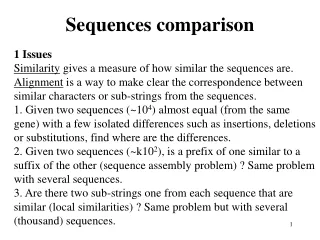
Sequences comparison
Sequences comparison. 1 Issues Similarity gives a measure of how similar the sequences are. Alignment is a way to make clear the correspondence between similar characters or sub-strings from the sequences.


Sequences comparison
E N D
Presentation Transcript
Sequences comparison 1 Issues Similarity gives a measure of how similar the sequences are. Alignment is a way to make clear the correspondence between similar characters or sub-strings from the sequences. 1. Given two sequences (~104) almost equal (from the same gene) with a few isolated differences such as insertions, deletions or substitutions, find where are the differences. 2. Given two sequences (~k102), is a prefix of one similar to a suffix of the other (sequence assembly problem) ? Same problem with several sequences. 3. Are there two sub-strings one from each sequence that are similar (local similarities) ? Same problem but with several (thousand) sequences.
2. Basic Algorithm 2. Basic Algorithm Sizes of the two sequences t and s may be different. Alignments produces two sequences issued from t and s whose sizes are equal by inserting spaces. It does not contain elementary alignment of spaces. Example: GA- CGGG-ATTA CATGCCGATTAG Score of an alignment: sum of the score of the elementary alignments. Example: +1 for a match, -1 for a mismatch, -2 for an indel (insertion-deletion). Similarity sim(s, t) is the maximal score possible between s and t.
Basic Algorithm (cont.1) Dynamic programming The problem is to determine sim(s, t) and a best alignment between s and t (such that its score value is sim(s, t)). Dynamic programming uses the so-called "composition principle": "the value (similarity) of the whole (couple of sequences) is a function of its parties". We use it to compute sim(s,t). This principle raises two questions (see Assignment1): 1. Into which parties have we to decompose a couple of sequences ? 2. Which is the function giving the similarity of a couple of sequence from the similarities of the parties ?
Basic Algorithm (cont.2) 1. An idea (see Assignment1) about the possible decompositions could be the three following ones (with suffixes of s and t being of sizes 1 or 0): - a couple (prefixs, prefixt) of prefixes of s and t such that the respective suffixes sufs and suft are letters (inducing an elementary alignment which is a match or a mismatch) . - a couple (prefixs, prefixt) of prefixes of s and t such that the suffix sufs is the voïd sequence and suft a letter (inducing an elementary alignment which is an indel, insertion or deletion) - a couple (prefixs, prefixt) of prefixes of s and t such that the suffix sufs is a letter and suft the voïd sequence (inducing an elementary alignment which is an indel) These decompositions avoid elementary alignments of spaces.
Basic Algorithm (cont.3) 2. For each decomposition, the required function is simply addition. Let be prefs = s[1...i-1], preft= t[1...j-1], then sim(s[1...i-1], t[1...j-1]) + p(i, j) where p(i, j) is the cost of a comparison between s[i] and s[j], gives the best score if using the first way of decomposing. To take into account the three possible decompositions, the function is : sim(s[1...i], t[1...j]) = max(sim(s[1...i-1], t[1...j-1]) + p(i, j), sim(s[1...i], t[1...j-1]) + g, sim(s[1...i-1], t[1...j]) + g)) with sim([], []) = 0 (it follows that sim([], t[1...j]) = j*g).
Basic Algorithm (cont.4) The computation uses a matrix a such that: a[i, j] = sim(s[1...i], t[1...j]) with 1 ≤ i ≤ m and 1 ≤ j ≤ n if m is the size of s and n the size of t. All the elements of the matrix a can be easily computed as a[i, j] is computed from a[i-1, j], a[i, j] and a[i, j-1]. The result is sim(s, t) = a[m, n]. Best alignments are paths (see Assignment1) constructed from a[m, n] to a[0, 0] which take optimal transitions between nodes (couples of prefixes). Each preceding nodes of a[i, j] can be computed by using the definition of sim (any choice can lead to a[0, 0]). Complexity: O(m*n) in time and space to compute similarities, O(m+n) to compute a best alignment. Be careful, searching for alignments could be exponential…
Local Comparison A local alignment between s and t is an alignment between a sub-string of t and a sub-string of s. We search for highest scoring local alignment. A sub-string of s is modeled as a suffix of a prefix of s. So, we have first to express the highest score highestscorepref(s[1...i], t[1...j]) between suffixes of prefixes of s and t. Note: suffixes of prefixes of s and t can be both void. Surprisingly, the definition of highestscorepref(s[1...i], t[1...j]) is very close to that one of sim(s[1...i], t[1...j]).
Local Comparison (cont.1) highestscorepref(s[1...i], t[1...j]) = max( highestscorepref (s[1...i-1], t[1...j-1]) + p(i, j), highestscorepref (s[1...i], t[1...j-1]) + g, highestscorepref (s[1...i-1], t[1...j]) + g), highestscorepref ([],[]) ) with highestscorepref ([],[]) = 0 (it follows that highestscorepref ([], t[1...j]) = 0) An highest scoring local alignment is constructed from node a[i, j] having the maximal value, in a way similar to the global case. The construction stops when a node of score 0 is reached.
Semi-global Comparison One does not consider spaces at the beginning(or the end) of an alignment. Examples: Alignment1: CAGCA- CTTGGATTCTCGG (from t) - - -CAGCGTGG- - - - - - - - - (from s) The score of alignment is-19. But if spaces at the beginning of s are not considered the score is –3. Another alignment has a better score (-12): Alignment2: CAGCACTTGGATTCTCGG (from t) CAGC - - - - - G- T - - - - GG (from s) In the case where end spaces are ignored after the last character of s the similarity between s and t becomes: sim(s,t) = maxj =1…n (a[m, j])
Semi-global Comparison (cont.1) In the case where end spaces are ignored after the last character of s, the similarity between s and t is the highest one between s and a prefix of t. Then : sim(s,t) = maxj =1…n (a[m, j]) In the case where beginning spaces of s are ignored, a[i, j] must contain the highest similarity between s[1…i] and a suffix of t[1…j]. Then the usual definition of sim(t, s) holds except that this time a[0, j] = 0. Exercice : How to proceed if one does not want to charge both beginning and end spaces of s and t ?
3. Extensions to the basic algorithm 1. Saving space The quadratic complexity is unavoidable. With respect to space, it possible to improve complexityfrom quadratic to linear. First, computing similarity can be easily done in linear space. We use a vector which contains at each step the line a[i-1, 0…j-1] and the line a[i, 0…j-1]. From this vector a[i, j] is easily computed. Computing best alignments is more difficult. Let be optimal(s, t) an optimal alignment. Then the composition principle can be applied by splitting s into three parts: s[1…i-1], s[i], s[I+1…m].
Saving space This principle induces that it exists j such that : optimal(s, t) = optimal(s[1…i-1], t[1…j-1]) . elementary_alignment(s[i], t[j]) . optimal(s[i+1…m], t[j+1…n]) or such that (by inserting a space in t): optimal(s, t) = optimal(s[1…i-1], t[1…j]) . elementary_aligment(s[i], -) . optimal(s[i+1…m], t[j+1…n]) So optimal(s, t) could be computed provided we know j.
Saving space (cont.1) Let simpreij (resp. simsufij) be the similarity between s[1…i-1] (resp. s[i+1…m]) and the prefixes terminating at position j (resp. suffixes beginning at position j) of t. The index j is such that: simpreij + score(s[i], t[j]) + simsufixij+1 or simpreij + score(s[i], -) + simsufixij is maximum. These similarities can be computed in linear space. Exercise: Show that processing time roughly doubles. Hints: Let T(m, n) be the number of times a maximum is computed for having the similarities. T(m, n) is proportional to the total processing time. Show that T(m, n) < 2*m*n. Note that T(1, n) 2*n (no maximum computations will occur).
General and affine gap penalty functions General gap penalty functions are such that the penalty for a block of size n is -w(n). w(k) could be different of b*k where b is the score of a gap (generally less than b*k). It could not be additive (sum of similarities of the components is not the similarity of the whole). The complexity becomes cubic. Less general functions (sub-additive functions)which satisfies w(k) kw(1) and w(k1 + …+kn) w(k1) + …+ w(kn) are affine functions of the form w(k) = h +gk (h>0, g >0) with k 1 and w(0) =0. The first space costs h + g and each following space costs g. Then the complexity remains quadratic.
Comparing similar sequences We treat the case where the two sequences have the same length n. Spaces will be inserted in pairs (one in s one in t). The number of space pairs k is greater than or equal to the maximum departure from the main diagonal. A narrow band around the main diagonal suffices to compute the optimal score alignment and alignments. The algorithm runs in time o(kn) which is a big win over the usual o(n2) if k is small compared to n.
Comparing similar sequences(cont.1) How to use K-band ? If a[n, n] is greater or equal to the best score that would be come from an alignment with k+1 pairs, an optimal alignment has been found with o(kn) steps. This best possible bs score is : M*(n-k-1) + 2(k+1)*g = bs where M (>0) is the score of a match and g ( 0) is added for each space.
Comparing similar sequences(cont.2) Exercise. Suppose that each time ak[n,n] < bs then k doubles and the algorithm is run again. Find a bound of the complexity of K-band in function n and sim(s, t). Observe that the complexity becomes better as the similarity grows. Hints: Express the stop condition for k and the non stop condition for k/2. Express the complexity and its bound depending whether ak[n, n] = ak/2[n, n] or ak[n, n] > ak/2[n, n].
Comparing multiple sequences • Multiple alignment : sequences are extended by inserting spaces in such a way as to make them all the same size. No column is made exclusively of spaces. • The SP-measure (Sum of Pairs): • To score a column we want a function with k arguments, where k is the number of sequences. One (impractical way) would be to implement this function as a k-dimensional array: if k =10 this would need 210 –1 > 1000 combinations. • Reasonable properties for a manageable function could be: • result independent from the order of the arguments (same sore for (V, V, I, -) and (I, I, V, -)). • penalization of unrelated residues and spaces
The SP-measure • A well-known function SP-score is such that: • SP-score(I, -, I, V) = p(I, -) + p(I, I) + p(I, V) • + p(-, I) + p(-, V) + p(I, V) • = SP-score(V, V, I, -) • Where p(a, b) is the pairwise score of symbols a and b. • It is possible to have two spaces in the same column. The common practice is to set p(-,-) = 0. • it is consistent with the induced pairwise alignment: elementary 2-alignments composed of spaces are removed. • it is compatible with SP-score() = i<j score(ij) where ij is the induced alignment on sequences i and j from alignment .
Dynamic programming approach • Cost in space: o(nk) for k sequences of length n. • Cost in time: • 2k –1 possible compositions to be examined at each step.(23-1 for 3 sequences). • SP-score method requires o(k2) steps by column (ie k(k-1)/2 pairs) • The total complexity is o(k2 2k nk) if S-score is used. • Exercise: Heuristics based on SP-scores for saving time which limit the positions (of the k-dimensional array) to those which are relevant to optimal alignments. • Hints: Suppose optimal. It could be that the induced 2-alignments are not optimal. But an idea based on the following one can be used: a position is relevant only if it belongs to all deduced optimal 2-alignments.
Star Alignment A sequence sc is chosen: the center of the star. 1. The goal is to get a multiple alignment such that all pairwise alignments ij where i or j is sc are optimal. The cost of all optimal pairwise alignments is o(kn2). 2. A multiple alignment is obtained by composing a multiple alignment (with sc) with a pairwise alignment (with sc) with the following approach: “one gap in sc, always a gap in sc”. Cost of a composition is o(kl) where l is the maximum length of the alignment. The total cost is o( k2l). Choice of sc: For example, such that i sim(si, sc) is maximized.
Tree Alignments • Data: k sequences, a (evolutionary) tree with k leaves, a one to one correspondence between sequences and leaves. • Tree alignment problem: We have to assign sequences to the interior nodes of the tree in such a way that the score of the tree is maximum. This score is the sum of the similarities between the sequences connected via an edge. • The star alignment is a particular case of tree alignment.
Tree Alignments Exercise: Consider a tree T with two leaves GAT and GT connected to and edge x and two leaves CG and CTG connected to an edge y, such that x and y are connected. Suppose x = CT and y = GC. Compute the score of the tree T in term of distances (more or less a dual notion of similarity). Consider the distance p(a, b) such that : p(a, b) = if a = b then 1 else 0 p(a, -) = -1 Which tree alignment could you deduce ?