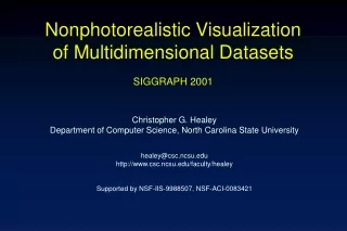
Nonphotorealistic Visualization of Multidimensional Datasets SIGGRAPH 2001
Nonphotorealistic Visualization of Multidimensional Datasets SIGGRAPH 2001 Christopher G. Healey Department of Computer Science, North Carolina State University healey@csc.ncsu.edu http://www.csc.ncsu.edu/faculty/healey Supported by NSF-IIS-9988507, NSF-ACI-0083421

Nonphotorealistic Visualization of Multidimensional Datasets SIGGRAPH 2001
E N D
Presentation Transcript
Nonphotorealistic Visualizationof Multidimensional DatasetsSIGGRAPH 2001 Christopher G. HealeyDepartment of Computer Science, North Carolina State Universityhealey@csc.ncsu.eduhttp://www.csc.ncsu.edu/faculty/healeySupported by NSF-IIS-9988507, NSF-ACI-0083421
Goals of Multidimensional Visualization • Effective visualization of large, multidimensional datasets • size: number of elements nin dataset • dimensionality: number of attributes membedded in each element • Display effectively multiple attributes at a single spatial location? • Rapidly, accurately, and effortlessly explore large amounts of data?
Visualization Pipeline Multidimensional Dataset • Dataset Management • Visualization Assistant • Perceptual Visualization • Nonphotorealistic Visualization• Assisted Navigation Perception
Formal Specification • Dataset D = { e1, …, en } containing n elements ei • D represents m data attributes A = { A1, …, Am } • Each ei encodes m attribute values ei = { ai,1, …, ai,m } • Visual features V = { V1, …, Vm } used to represent A • Function j: Aj Vj maps domain of Aj to range of displayable values in Vj • Data-feature mapping M( V, F ), a visual representation of D • Visualization: Selection of M and viewers interpretation of images produced by M
Temperature Windspeed Precipitation Pressure Separate Displays n = 42,224 elementsm = 4A1 = temperatureA2 = windspeedA3 = precipitationA4 = pressureV = colour F = dark blue bright pink
Integrated Display n = 42,224 elementsm = 4A1 = temperatureA2 = windspeedA3 = precipitationA4 = pressureV1 = colourV2 = sizeV3 = orientationV4 = density F1 = dark blue bright pink F2 = 0.25 1.15 F3 = 0º 90º F4 = 1x1 3x3
Cognitive Vision • Psychological study of the human visual system • Perceptual (preattentive) features used to perform simple tasks in < 200 milliseconds • features: hue, intensity, orientation, size, length, curvature, closure, motion, depth of field, 3D cues • tasks:target detection, boundary detection, region tracking, counting and estimation • Perceptual (preattentive) tasks performed independent of display size • Develop, extend, and apply results to visualization
A B A B C D E F Effective Hue Selection • How can we choose effectively multiple hues? • Suppose: { A, B } Suppose: { A, B, C, D, E, F } • Rapidly and accurately identifiable colors? • Equally distinguishable colors? • Maximum number of colors? • Three selection criteria: color distance, linear separation, color category
Colour Distance B A C CIE LUV isoluminant slice; AB = AC implies equal perceived colour difference
Linear Separation A C T B Without linear separation (T in A & B, harder) vs. with linear separation (T in A & C, easier)
Colour Category green A red T B blue purple Between named categories (T & B, harder) vs. within named categories (T & A, easier)
Distance / Linear Separation Y d GY l R d B P Constant linear separation l, constant distance d to two nearest neighbours
Example Experiment Displays 3 colours17 elements 7 colours49 elements Target: red square; 3-colour, 17 element displays and 7-colour, 49 element displays
Perceptual Texture Elements • Design perceptual texture elements (pexels) • Pexels support variation of perceptual texture dimensions height, density, regularity • Attach a pexel to each data element • Element attributes control pexel appearance • Psychophysical experiments used to measure: • perceptual salience of each texture dimension • visual interference between texture dimensions
Pexel Examples Height Regularity Density
Results • Subject accuracy used to measure performance • Taller pexels identified preattentively with no interference (93% accuracy) • Shorter, denser, sparser identified preattentively • Some height, density, regularity interference • Irregulardifficult to identify (76% accuracy); height, density interference • Regular cannot be identified (50% accuracy)
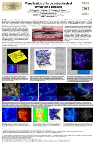
Typhoon Visualization n = 572,474m = 3 A1 = windspeed;A2 = pressure;A3 = precipitation V1 = height;V2 = density;V3 = color f1 = short tall; f2 = dense sparse; f3 = blue purple Typhoon Amber approaches Taiwan, August 28, 1997
Typhoon Visualization n = 572,474m = 3A1 = windspeed;A2 = pressure;A3 = precipitation V1 = height;V2 = density;V3 = color f1 = short tall; f2 = dense sparse; f3 = blue purple Typhoon Amber strikes Taiwan, August 29, 1997
Impressionism • Underlying principles of impressionist art: • Object and environment interpenetrate • Colour acquires independence • Show a small section of nature • Minimize perspective • Solicit a viewer’s optics • Hue, luminance, color explicitly studied and controlled • Other stroke and style properties correspond closely to low-level visual features • path, length, energy, coarseness, weight • Can we bind data attributes with stroke properties? • Can we use perception to control painterly rendering?
Water Lilies (The Clouds) 1903; Oil on canvas, 74.6 x 105.3 cm (29 3/8 x 41 7/16 in); Private collection
Rock Arch West of Etretat (The Manneport) 1883; Oil on canvas, 65.4 x 81.3 cm (25 3/4 x 32 in); Metropolitan Museum of Art, New York
Wheat Field 1889; Oil on canvas, 73.5 x 92.5 cm (29 x 36 1/2 in); Narodni Galerie, Prague
Gray Weather, Grande Jatte 1888; Oil on canvas, 27 3/4 x 34 in; Philadelphia Museum of Art. Walter H. Annenberg Collection
StrokeFeature Correspondence • Close correspondence between Vj and Sj • hue color, luminance lighting, contrast density, orientation path, area size • ei in D analogous to brush strokes in a painting • To build a painterly visualization of D: • construct M( V, F ) • map Vj in V to corresponding painterly styles Sj in S • M now maps ei to brush strokes bi • ai,j in ei control painterly appearance of bi
Eastern US, January n = 69,884m = 4 A1 = temperature;A2 = windspeed;A3 = pressure;A4 = precipitation V1 = color;V2 = density;V3 = size;V4 = orientation f1 = blue pink; f2 = sparse dense; f3 = small large;f4 = upright flat
Rocky Mountains, January n = 69,884m = 4 A1 = temperature;A2 = windspeed;A3 = pressure;A4 = precipitation V1 = color;V2 = density;V3 = size;V4 = orientation f1 = blue pink; f2 = sparse dense; f3 = small large;f4 = upright flat
Pacific Northwest, February n = 69,884m = 4 A1 = temperature;A2 = windspeed;A3 = pressure;A4 = precipitation V1 = color;V2 = density;V3 = size;V4 = orientation f1 = blue pink; f2 = sparse dense; f3 = small large;f4 = upright flat
Conclusions • Formalisms identify a visual feature painterly style correspondence • Can exploit correspondence to construct perceptually salient painterly visualizations • Recent and future work + psychophysical experiments confirm perceptual guidelines extend to painterly environment • subjective aesthetics experiments • improved computational models of painterly images • additional painterly styles • dynamic paintings (e.g., flicker, direction and velocity of motion)