AN IFORMATION THEORETIC APPROACH TO BIT STUFFING FOR NETWORK PROTOCOLS
410 likes | 595 Vues
AN IFORMATION THEORETIC APPROACH TO BIT STUFFING FOR NETWORK PROTOCOLS. Jack Keil Wolf Center for Magnetic Recording Research University of California, San Diego La Jolla, CA DIMACS Workshop on Network Information Theory Rutgers University March 17-19, 2003. Acknowledgement.

AN IFORMATION THEORETIC APPROACH TO BIT STUFFING FOR NETWORK PROTOCOLS
E N D
Presentation Transcript
AN IFORMATION THEORETIC APPROACH TO BIT STUFFING FOR NETWORK PROTOCOLS Jack Keil Wolf Center for Magnetic Recording Research University of California, San Diego La Jolla, CA DIMACS Workshop on Network Information Theory Rutgers University March 17-19, 2003
Acknowledgement • Some of this work was done jointly with: Patrick Lee Paul Bender Sharon Aviran Jiangxin Chen Shirley Halevy (Technion) Paul Siegel Ron Roth (Technion)
Constrained Sequences and Network protocols • In many protocols, specific data patterns are used as control signals. • These prohibitedpatterns must be prevented from occurring in the data. • In any coding scheme that prohibits certain patterns from occurring, the number of constrained (or coded) bits must exceed the number of data bits.
Relationship to Information Theory • The average number of data bits per constrained bit is called the rate of the code. • The Shannon capacity is the maximum rate of any code. • Practical codes usually have rates strictly less than the Shannon capacity.
Bit Stuffing • Bit stuffing is one coding technique for preventing patterns from occurring in data. • The code rate for bit stuffing is always less than the Shannon capacity. • Here we show how to make the code rate for bit stuffing equal to the Shannon capacity.
Bit Stuffing and Protocols • Definition from Webopedia: (http://www.webopedia.com/TERM/B/bit_stuffing.html) “bit stuffing-The practice of adding bits to a stream of data. Bit stuffing is used by many network and communication protocols for the following reasons: To prevent data being interpreted as control information. For example, many frame-based protocols, such as X.25, signal the beginning and end of a frame with six consecutive 1’s. Therefore, if the actual data has six consecutive 1 bits in a row, a zero is inserted after the first 5 bits…Of course, on the receiving end, the stuffed bits must be discarded…” data:01111110111110101010… This won’t work: transmit: 011111010111110101010… But this will: transmit: 0111110101111100101010…
A Diversion: Binary (d,k) Constrained Sequences • The X.25 constraint is a special case of a binary (d,k) constraint used in digital storage systems. • Such binary sequences have at least d and at most k 0’s between adjacent 1’s. • For d > 0 and finitek, the sequences are produced by the edge labels when taking tours of the graph: 0 0 1 0 0 d-1 0 d 0 d+1 0 … 0 k-1 0 k … 1 1 1 1
Binary (0,k) Constrained Sequences • For d=0 and finitek, allowable sequences are produced by the edge labels of the graph: 1 0 0 0 0 0 0 1 2 k-1 k 1 1 1 1
Binary (d,∞) Constrained Sequences • For infinitek, the sequences are produced by the edge labels when touring the graph: 0 0 0 0 0 0 0 1 2 d-1 d 1
Back to Protocols • By complementing the bits in a (0,5) code, we will produce sequences that have no more than 5 consecutive 1’s. • Thus, after complementing the bits, any (0,5) code can be used in the X25 protocol.
Bit Stuffing • In this talk we will investigate the code rates which can be achieved with bit stuffing and compare these rates with the Shannon capacity. • We will use as our constraint, binary (d,k) codes, although our technique applies to a much wider class of codes. • We will begin with plain vanilla bit stuffing which gives rates strictly less than capacity. • Then we show how bit stuffing can be modified to yield rates equal to capacity for some values of d and k. • Finally we show how bit stuffing can be further modified to yield rates equal to capacity for all values of d and k.
Bit Stuffing for (d,k) Codes • For any value of d and k (0 < d < k), one can use bit stuffing to form sequences that satisfy the constraint. • The bit stuffing encoding rule is: Step 1. If last bit is a 1, stuff d 0’s. Go to next step. (Skip this step if d=0.) Step 2. If last k bits are 0’s stuff a 1. Return to first step. (Skip this step if k=∞.) 0 0 0 0 0 1 d-1 d 0 d+1 0 … 0 k-1 0 k … 1 1 1 1
Rate for Bit Stuffing vs Shannon Capacity of (d,k) Codes • The rate for bit stuffing is the average number of information bits per transmitted symbol. • The rate here is computed for i.i.d. binary data with equally likely 0’s and 1’s. • The Shannon capacity of a (d,k) constrained sequence is the maximum rate of any encoder-decoder that satisfies the constraint. • Therefore the rate for bit stuffing is less than or equal to the Shannon capacity of the constraint.
Shannon Capacity of a (d,k) Constraint • Define N(n) as the number of distinct binary sequences oflength n that satisfy the constraint. • Then, for every 0 < d < k, exists and is called the Shannon capacity of the code.
Shannon Capacity • Shannon (1948) gave several methods for computing the capacity of (d,k) codes. • For finite k, he showed that the following difference equation describes the growth of N(n) with n: N(n)=N(n-(d+1))+N(n-(d+2))+ … +N(n-(k+1)). • By solving this difference equation, Shannon showed that the capacity, C = C(d,k), is equal to the base 2logarithm of the largest real root of the equation: xk+2 - xk+1 - xk-d+1 +1 = 0.
Bit Stuffing and Shannon Capacity • If one uses bit stuffing on uncoded data, except for ` the trivial case of (d=0, k=∞), the rate always is strictly less than the Shannon capacity. • The rate here is computed for i.i.d. binary data with equally likely 0’s and 1’s. • But by a modification to bit stuffing, using a distribution transformer, we can improve the rate and sometimes achieve capacity.
Slight Modification to Bit Stuffing • A distribution transformer converts the binary data sequence into an i.i.d. binary sequence that is p- biased for 0 < p < 1. The probability of a 1 in this biased stream is equal to p. • The distribution transformer can be implemented by a sourcedecoder for a p-biased stream. • The conversion occurs at a rate penalty h(p), where h(p) = -plog(p)-(1-p)log(1-p). • We can choose p to maximize the code rate and sometimes achieve capacity.
Bit Stuffing with Distribution Transformer 1-p p ½½ Distribution Transformer p-Bias 0 1 0 0 1 … 0 0 1 1 0 … Distribution Transformer p-Bias Bit Stuffer 10001010000010000 … 010011100101 … 1000110000000 ... Inverse Distribution Transformer Bit Unstuffer 10001010000010000 … 010011100101 … 1000110000000 ...
Slight Modification to Bit Stuffing • As shown by Bender and Wolf, after optimizing p, the code rate can be made equal to theShannon capacity for the cases of (d, d+1) and (d,∞), sequences for every d > 0. • However, even after choosing the optimum value of p, the code rate is strictly less than the Shannon capacity for all other values of d and k.
Code Rate vs. p (B&W) 0 0.5 1.0
Two Questions • Why does this technique achieve capacity only for the cases: k = d+1 and k = ∞? • Is it possible to achieve capacity for other cases? • To answer these questions we make a slight diversion.
A Further Diversion: Bit Stuffing and 2-D Constraints • Bit stuffing has been used to generate two dimensional constrained arrays. • Details of this work are in a series of papers, the latest entitled “Improved Bit-Stuffing Bounds on Two-Dimensional Constraints” which has been submitted to the IEEE Transactions on Information Theory by: Shirley Halevy Technion Jiangxin Chen UCSD Ron Roth Technion Paul Siegel UCSD Me UCSD
Two Dimensional Constraints • Two dimensional constrained arrays can have applications in page oriented storage. • These arrays could be defined on different lattices. Commonly used are the rectangular lattice and the hexagonal lattice. • Example 1: Rectangular lattice with a (1, ∞) constraints on the rows and columns: 0 0 1 0 0 • Example 2: Hexagonal lattice with a (1, ∞) constraints in 3 directions: 0 0 0 1 0 0 0
Capacity and Two Dimensional Constrained Arrays • Calculating the Shannon capacity for two dimensional constrained arrays is largely an open problem. • The exact value of the capacity for the rectangular (1, ∞) constraint is not known. However, Baxter has obtained the exact value of the capacity of the hexagonal (1, ∞) constraint. • In some cases where the two dimensional capacity is not known, we have used bit stuffing to obtain tight lower bounds to the capacity.
Two Dimensional Bit Stuffing: Rectangular Lattice with (1, ∞) Constraint • A distribution transformer is used to produce a p- biased sequence. • The p-biased sequence is written on diagonals • Every time a p-biased 1 is written, a 0 is inserted (that is stuffed) to the right and below it. • In writing the p-biased sequence on diagonals, the positions in the array containing stuffed 0’s are skipped.
Bit Stuffing and Two Dimensional Constrained Arrays • Suppose we wish to write the p-biased sequence 01 02 03 14 05 06 17 08 … 01 02 14 04 03 05 04 06 17 07 08 07
“Double Stuffing” with the (1, ∞) Constraint • Sometimes a p-biased 1 results in only one stuffed 0 since there is already a stuffed 0 to the right of it. • In writing the sequence 01 02 03 14 15 06 07 …, 15 results in only a single stuffed 0, since 14 having been written above and to the right of it, already has written the other 0. That is, 04,5 is a “double” stuffed 0. 01 02 1404 03 15 04,5 0605 07
Multiple p-Biased Transformers • This suggests having two values for p: one, p0, for the case where the bit above and to the right of it is a 0 and the other, p1, when that bit is a 1. • Doing this and optimizing we obtain: p0= 0.328166 p1=0.433068 code rate=0.587277 (which is within 0.1% of capacity) • This suggests using multiple p’s in one dimension to improve the code rate.
Shannon Capacity and Edge Probabilities • The maximum entropy (i.e., the capacity) of a constraint graph induces probabilities on the edges of the graph. • For finite k, the Shannon capacity is achieved when the edges of the graph are assigned the probabilities as indicated below where C = log(l). 1-{l-(d+2) / (1-l-(d+1))} (1-l-(d+1)) 1 1 1 1 1 0 1 2 d-1 d d+1 d+2 k l-(d+1) 1 l-(d+2) / (1-l-(d+1))
Shannon Capacity and Edge Probabilities • And for the (d, ∞) constraint, the Shannon capacity is achieved when the edges of the graph are assigned the probabilities as indicated: 1-l-(d+1) 1 1 1 1 1 0 1 2 d-1 d l-(d+1)
Why Bit Stuffing Sometimes Achieved Capacity for B&W • The graphs for the two cases of constraints that achieved capacity are shown below : • Note that for both graphs, only one state has two edges emanating from it. Thus, only one bias suffices and the optimum p for both cases is: p= l-(d+1). • For other values of d and k, there will be more than one state with two exiting edges. 1-l-(d+1) 1-l-(d+1) 1 1 1 1 l-(d+1) l-(d+1) 1 (d, ∞) Constraint (d,d+1) Constraint
Capacity Achieving Bit Stuffing • This suggests a better scheme which achieves capacity for all values of d and k. • For k finite, there are (k-d) states in the graph with two protruding edges. • The binary data stream is converted into (k-d) data streams, each by a different distribution transformer. The p’s of each of the transformers are chosen to emulate the maxentropic edge probabilities for the the (k-d) states with two protruding edges.
Block Diagram of Encoder Distribution Transformer pd-Bias Smart DeMux Distribution Transformer Pd+1-Bias Bit Stuffer Smart Mux Distribution Transformer p(k-1)-Bias
Bit Stuffing with Average Rate Equal to the Shannon Capacity • Example: (1,3) Code The maxentropic probabilities for the branches are: Thus, one distribution transformer should have p=0.4655 and the second distribution transformer should have p=0.5943. 1 0.5345 0.4057 Run Length Probabilities Length Probability 2 0.4655 3 0.3176 4 0.2167 1 0.4655 0.5943
Bit Stuffing with Average Rate Equal to the Shannon Capacity • Example: (2,4) Code The maxentropic probabilities for the branches are: Thus, one distribution transformer should have p=0.4301 and the second distribution transformer should have p=0.5699. But only one distribution transformer is needed. Why? 1 1 0.5699 0.4301 Run Length Probabilities Length Probability 3 0.4301 4 0.3247 5 0.2451 1 0.4301 0.5699
Bit Flipping and Bit Stuffing • For the (2,4) case, one can use one distribution transformer and bit flipping in conjunction with bit stuffing to achieve capacity. • For k finite, we next examine such a system for arbitrary (d,k): Distribution Transformer p-Bias Controlled Bit Flipper Bit Stuffer
Questions • What is the optimal bit flipping position? • When can we improve the rate by bit flipping? • Can we achieve capacity for more constraints, using bit flipping? • If not, how far from capacity are we? 1-p 1-p p p 1 1 1-p p 0 1 d d+1 ?? k-1 k . . . . . . . . . p p 1-p 1-p 1
Answers (Aviran) • For all (d,k) with d≥1, d+2≤k<∞ and p<0.5: • theoptimal flipping position is k-1. • For all (d,k) with d≥1, d+2≤k<∞: • flipping improves the rate over original bit stuffing. • Capacity is achieved only for the (2,4) case. 1 1 1-p 1-p 1-p 1-p p 0 1 d d+1 k-2 k-1 k . . . . . . p p p 1 1-p
Topics Missing From This Talk • A lot of interesting mathematics. • Results for more general one and two dimensional constraints. • A list of unsolved problems.