CE 400 Honors Seminar Molecular Simulation
300 likes | 618 Vues
CE 400 Honors Seminar Molecular Simulation. Class 4. Prof. Kofke Department of Chemical Engineering University at Buffalo, State University of New York. Statistical Mechanics. Theoretical basis for derivation of macroscopic behaviors from microscopic origins

CE 400 Honors Seminar Molecular Simulation
E N D
Presentation Transcript
CE 400 Honors SeminarMolecular Simulation Class 4 Prof. Kofke Department of Chemical Engineering University at Buffalo, State University of New York
Statistical Mechanics • Theoretical basis for derivation of macroscopic behaviors from microscopic origins • Two fundamental postulates of equilibrium statistical mechanics • microstates of equal energy are equally likely • time average is equivalent to ensemble average • Formalism extends postulates to more useful situations • thermal, mechanical, and/or chemical equilibrium with reservoirs • systems at constant T, P, and/or m • yields new formulas for probabilities of microstates • derivation invokes thermodynamic limit of very large system • Macroscopic observables given as a weighted sum over microstates • dynamic properties require additional formalism
Ensembles • Definition of an ensemble • Collection of microstates subject to at least one extensive constraint • “microstate” is specification of all atom positions and momenta • fixed total energy, total volume, and/or total number of molecules • unconstrained extensive quantities are represented by full range of possible values • Probability distribution p describing the likelihood of observing each state, or the weight that each state has in ensemble average • Example: Some members of ensemble of fixed N • isothermal-isobaric (TPN) • all energies and volumes represented Low-probability state
Markov Processes 1. • Stochastic process • movement through a series of well-defined states in a way that involves some element of randomness • for our purposes,“states” are microstates in the governing ensemble • Markov process • stochastic process that has no memory • selection of next state depends only on current state, and not on prior states • process is fully defined by a set of transition probabilities pij • pij = probability of selecting state j next, given that presently in state i. • Transition-probability matrix P collects all pij • Application • we can visit the states of a system in proportion to their probability by application of a Markov process
Transition-Probability Matrix • Example • system with three states • Requirements of transition-probability matrix • all probabilities non-negative, and not greater than unity • sum of each row is unity • probability of staying in present state may be non-zero If in state 1, will stay in state 1 with probability 0.1 If in state 1, will move to state 3 with probability 0.4 Never go to state 3 from state 2
Example • Here’s a transition-probability matrix for an eight-state system • Let’s do a walk based on it…
Distribution of State Occupancies 2 1 3 • Consider process of repeatedly moving from one state to the next, choosing each subsequent state according to P • 1 22132233123 etc. • Histogram the occupancy number for each state • n1 = 3 p1= 0.33 • n2 = 5p2 = 0.42 • n3 = 4 p3 = 0.25 • After very many steps, a limiting distribution emerges • Click here for an applet that demonstrates a Markov process and its approach to a limiting distribution
Microscopic Reversibility • The limiting distribution and the transition probabilities obey the principle of microscopic reversibility, a.k.a., detailed balance • Loosely: “net flow from state i to state j equals net flow from state j to state i” • Consider the example • Limiting distribution:
Application? • How does this apply to molecular simulation? • Statistical mechanics provides the limiting distribution • Canonical ensemble • The Markov process relates the limiting distribution and the transition probabilities • What is needed to tie these together? • How can it be done?
Metropolis Algorithm • Standard method to form Markov process in molecular simulation • Metropolis, Rosenbluth, Rosenbluth, Teller and Teller, Journal of Chemical Physics, 21, 1087 (1953). • Transition probabilities formulated to yield desired limiting distribution • Each Markov transition is a two-step process • From state i select a trial state j with probability Tij • Accept trial with probability c: • Generate a uniform random deviate r on (0,1) • If r < c, accept, otherwise reject and use previous state as next one • With this recipe • Show that this obeys detailed balance
Monte Carlo Simulation State k • MC techniques applied to molecular simulation • Almost always involves a Markov process • move to a new configuration from an existing one according to a well-defined transition probability • Simulation procedure • generate a new “trial” configuration by making a perturbation to the present configuration • accept the new configuration based on the ratio of the probabilities for the new and old configurations, according to the Metropolis algorithm • if the trial is rejected, the present configuration is taken as the next one in the Markov chain • repeat this many times, accumulating sums for averages State k+1
Trial Moves • A great variety of trial moves can be made • Basic selection of trial moves is dictated by choice of ensemble • almost all MC is performed at constant T • no need to ensure trial holds energy fixed • must ensure relevant elements of ensemble are sampled • all ensembles have molecule displacement, rotation; atom displacement • isobaric ensembles have trials that change the volume • grand-canonical ensembles have trials that insert/delete a molecule • Significant increase in efficiency of algorithm can be achieved by the introduction of clever trial moves • reptation, crankshaft moves for polymers • multi-molecule movements of associating molecules • many more
General Form of Algorithm Entire Simulation Initialization Reset block sums “cycle” or “sweep” New configuration “block” moves per cycle Add to block sum cycles per block Compute block average blocks per simulation Compute final results Monte Carlo Move New configuration Select type of trial move each type of move has fixed probability of being selected Move each atom once (on average) 100’s or 1000’s of cycles Independent “measurement” Perform selected trial move Decide to accept trial configuration, or keep original
Displacement Trial Move 1. Specification • Gives new configuration of same volume and number of molecules • Basic trial:
Displacement Trial Move 1. Specification • Gives new configuration of same volume and number of molecules • Basic trial: • displace a randomly selected atom to a point chosen with uniform probability inside a cubic volume of edge 2d centered on the current position of the atom Select an atom at random
Displacement Trial Move 1. Specification • Gives new configuration of same volume and number of molecules • Basic trial: • displace a randomly selected atom to a point chosen with uniform probability inside a cubic volume of edge 2d centered on the current position of the atom 2d Consider a region about it
Displacement Trial Move 1. Specification • Gives new configuration of same volume and number of molecules • Basic trial: • displace a randomly selected atom to a point chosen with uniform probability inside a cubic volume of edge 2d centered on the current position of the atom Consider a region about it
Displacement Trial Move 1. Specification • Gives new configuration of same volume and number of molecules • Basic trial: • displace a randomly selected atom to a point chosen with uniform probability inside a cubic volume of edge 2d centered on the current position of the atom Move atom to point chosen uniformly in region
Displacement Trial Move 1. Specification • Gives new configuration of same volume and number of molecules • Basic trial: • displace a randomly selected atom to a point chosen with uniform probability inside a cubic volume of edge 2d centered on the current position of the atom Consider acceptance of new configuration ?
Displacement Trial Move 1. Specification • Gives new configuration of same volume and number of molecules • Basic trial: • displace a randomly selected atom to a point chosen with uniform probability inside a cubic volume of edge 2d centered on the current position of the atom • Limiting probability distribution • canonical ensemble • for this trial move, probability ratios are the same in other common ensembles, so the algorithm described here pertains to them as well Examine underlying transition probabilities to formulate acceptance criterion ?
2. Analysis of Trial Probabilities • Detailed specification of trial moves and probabilities Forward-step trial probability Reverse-step trial probability v = (2d)d c is formulated to satisfy detailed balance
3. Analysis of Detailed Balance Forward-step trial probability Reverse-step trial probability pi pij pj pji Detailed balance = Limiting distribution
3. Analysis of Detailed Balance Forward-step trial probability Reverse-step trial probability pi pij pj pji Detailed balance = Limiting distribution
3. Analysis of Detailed Balance Forward-step trial probability Reverse-step trial probability pi pij pj pji Detailed balance = Acceptance probability
4a. Examination of Java Code public void thisTrial(Phase phase) { double uOld, uNew; if(phase.atomCount==0) {return;} //no atoms to move int i = (int)(rand.nextDouble()*phase.atomCount); //pick a random number from 0 to N-1 Atom a = phase.firstAtom(); for(int j=i; --j>=0; ) {a = a.nextAtom();} //get ith atom in list uOld = phase.potentialEnergy.currentValue(a); //calculate its contribution to the energy a.displaceWithin(stepSize); //move it within a local volume phase.boundary().centralImage(a.coordinate.position()); //apply PBC uNew = phase.potentialEnergy.currentValue(a); //calculate its new contribution to energy if(uNew < uOld) { //accept if energy decreased nAccept++; return; } if(uNew >= Double.MAX_VALUE || //reject if energy is huge or doesn’t pass test Math.exp(-(uNew-uOld)/parentIntegrator.temperature) < rand.nextDouble()) { a.replace(); //...put it back in its original position return; } nAccept++; //if reached here, move is accepted } Have a look at a simple MC simulation applet
4b. Examination of Java Code public final void displaceWithin(double d) { workVector.setRandomCube(); displaceBy(d,workVector);} public final void displaceBy(double d, Space.Vector u) { rLast.E(r); translateBy(d,u);} public final void translateBy(double d, Space.Vector u) {r.PEa1Tv1(d,u);} public final void replace() {r.E(rLast);} public void setRandomCube() { x = random.nextDouble() - 0.5; y = random.nextDouble() - 0.5; } public void E(Vector u) {x = u.x; y = u.y;} public void PEa1Tv1(double a1, Vector u) { x += a1*u.x; y += a1*u.y;} • Atom methods • Space.Vector methods
5. Tuning • Size of step is adjusted to reach a target rate of acceptance of displacement trials • typical target is 50% • for hard potentials target may be lower (rejection is efficient) Large step leads to less acceptance but bigger moves Small step leads to less movement but more acceptance
Assignments Summary • 0. Send me an email • completed • 1. Construct and deploy a simple molecular simulation applet • completed • 2. Find and review an article from the literature that applies molecular simulation • 10/9: Notify me of paper to examine • 10/16: Present 15-minute oral summary to class • 3. Design, construct, test and deploy a molecular simulation • Must demonstrate a non-trivial collective behavior • Incorporation of game-like features is encouraged • 10/23: Specification of simulation project due; prepare one design and an alternate in case of project duplication. In-class discussion of needed components by each group to complete their project. • 12/4: Present and explain applets in class
In-class Exercise • Construct a NPT Monte Carlo simulation • Lennard-Jones potential • Slider to adjust pressure • Meter and box display to show density • Measure density for several pressures • Use Lennard-Jones system of units • Construct a NVT Monte Carlo simulation • NSelector to select density • MeterPressureSoft and box display to show density • www.cheme.buffalo.edu/courses/ce400/MeterPressureSoft.class • Measure pressure for several densities • Compare results. Do pressure/density data agree?