Download
1 / 23
270 likes | 644 Vues
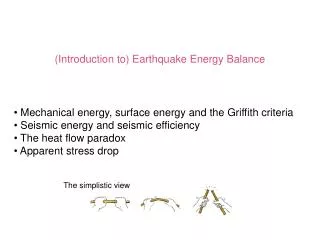
(Introduction to) Earthquake Energy Balance. Mechanical energy, surface energy and the Griffith criteria Seismic energy and seismic efficiency The heat flow paradox Apparent stress drop. The simplistic view. Earthquake energy balance: related questions.

E N D
(Introduction to) Earthquake Energy Balance • Mechanical energy, surface energy and the Griffith criteria • Seismic energy and seismic efficiency • The heat flow paradox • Apparent stress drop The simplistic view
Earthquake energy balance: related questions • Are faults weaker or stronger than the surrounding crust? • Do earthquakes release most, or just a small fraction of the strain energy that is stored in the crust?
Earthquake energy balance: Griffith criteria crack extends if: crack at equilibrium if crack heals if: The static frictionless case: • UM is the mechanical energy. • UA is the potential energy of the external load applied on the system boundary. • UE is the internal elastic strain energy stored in the medium • US is the surface energy.
Earthquake energy balance: dynamic shear crack Dynamic shear crack: • Here, in addition to UA, UE and US: • UK is the kinetic energy. • UF is the work done against friction. During an earthquake, the partition of energy (after less before) is as follows: where ES is the radiated seismic energy.
Earthquake energy balance: dynamic shear crack Since earthquake duration is so small compared to the inter seismic interval, the motion of the plate boundaries far from the fault is negligible, and UA=0. Thus, the expression for the radiated energy simplifies to: Question: what are the signs of UE, US and UF? Let us now write expressions for UE , US and UF .
Earthquake energy balance: elastic strain energy To get a physical sense of what UE is, it is useful to consider the spring-slider analog. The reduction in the elastic strain energy stored in the spring during a slip episode is just the area under the force versus slip curve. For the spring-slider system, UE is equal to:
Earthquake energy balance: elastic strain energy Similarly, for a crack embedded within an elastic medium, UE is equal to: where 1 and 2 are initial and final stresses, respectively, and the minus sign indicates a decrease in elastic strain energy.
Earthquake energy balance: frictional dissipation and surface energy The frictional dissipation: where F is the friction, V is sliding speed, and t is time. Frictional work is converted mainly to heat. The surface energy: where is the energy per unit area required to break the atomic bonds, and A is the rapture dimensions. Experimental studies show that is very small, and thus surface energy is very small compared to the radiated energy (but not everyone agrees with this argument).
Earthquake energy balance: the simplest model Consider the simplest model, in which the friction drops instantaneously from 1 to 2. In such case: F=2, and we get:
Earthquake energy balance: seismic efficiency We define seismic efficiency, , as the ratio between the seismic energy and the negative of the elastic strain energy change, often referred to as the faulting energy. which leads to: with being the static stress drop. While the stress drop may be determined from seismic data, absolute stresses may not.
Earthquake energy balance: seismic efficiency For small earthquakes, and . Combining this with the expression for seismic moment we get: Both M and r may be inferred from seismic data. The static stress drop is equal to: where G is the shear modulus, C is a geometrical constant, and (the tilde) L is the rupture characteristic length. The characteristic rupture length scale is different for small and large earthquakes.
Earthquake energy balance: seismic efficiency Stress drops vary between 0.1 and 10 MPa over a range of seismic moments between 1018 and 1027 dyn cm. Figure from: Schlische et al., 1996
Earthquake energy balance: seismic efficiency constraints on absolute stresses: In a hydrostatic state of stress, the friction stress increases with depth according to: where is the coefficient of friction, g is the acceleration of gravity, and c and w are the densities of crustal rocks and water, respectively. Laboratory experiments show: Byerlee, 1978
Earthquake energy balance: seismic efficiency Using: , the coefficient of friction = 0.6 c, rock density = 2600 Kg m-3 w, water density = 1000 Kg m-3 g, the acceleration of gravity = 9.8 m s-2 D, the depth of the seismogenic zone, say 12x103 m We get an average friction of: and the inferred seismic efficiency is:
Earthquake energy balance: seismic efficiency So, the radiated energy makes only a small fraction of the energy that is available for faulting. Based on this conclusion a strong heat-flow anomaly is expected at the surface right above seismic faults.
Earthquake energy balance: the heat flow paradox At least in the case of the San-Andreas fault in California, the expected heat anomaly is not observed. A section perpendicular to the SAF plane: Figure from: Scholz, 1990 The disagreement between the expected and observed heat-flow profiles is often referred to as the HEAT FLOW PARADOX.
Earthquake energy balance: the heat flow paradox A section parallel to the SAF plane: Figure from: Scholz, 1990
Earthquake energy balance • The assumptions underlying the ''simple model'' are: • Instantaneous drop from static to kinetic friction, and constant friction during slip. • Uniform distribution of slip and stresses. • Zero overshoot. • Constant sliding velocity. • No off fault deformation. • The first point means that continuity is violated...
Earthquake energy balance Other conceptual models: constant friction slip weakening quasi-static • The simple model. • The slip-weakening model. Significant amount of energy is dissipated in the process of fracturing the contact surface. In the literature this energy is interchangeably referred to as the break-up energy, fracture energy or surface energy. • A silent (or slow) earthquake - no energy is radiated.
Earthquake energy balance In reality, things are probably more complex than that. We now know that the distribution of slip and stresses is highly heterogeneous, and that the source time function is quite complex.
Earthquake energy balance: radiated energy versus seismic moment and the apparent stress drop Radiated energy and seismic moment of a large number of earthquakes have been independently estimated. It is interesting to examine the radiated energy and seismic moment ratio. Figure from: Kanamori, Annu. Rev. Earth Planet. Sci., 1994
Earthquake energy balance: radiated energy versus seismic moment and the apparent stress drop Remarkably, the ratio of radiated energy to seismic moment is fairly constant over a wide range of earthquake magnitudes. Figure from: Figure from Kanamori and Brodsky, Rep. Prog. Phys., 2004
Earthquake energy balance: radiated energy versus seismic moment and the apparent stress drop What is the physical interpretation of the ratio ES to M0? Recall that the seismic moment is: and the radiated energy for constant friction (i.e., F = 2): Thus, ES/M0 multiplied by the shear modulus, G, is simply: This is often referred to as the 'apparent stress drop'.