Overview of ANOVA
Overview of ANOVA. ANOVA. Analysis of variance IV referred to as a factor Conditions also called level or treatment, with k representing the number of levels Thus, refer to as treatment effect One-way ANOVA. Why ANOVA ?.

Overview of ANOVA
E N D
Presentation Transcript
ANOVA • Analysis of variance • IV referred to as a factor • Conditions also called level or treatment, with k representing the number of levels • Thus, refer to as treatment effect • One-way ANOVA
Why ANOVA ? • Many versions applied to lots of experimental designs, especially complex designs with more than one IV • Goes beyond the basic t-test when have more than 2 levels, MUST use ANOVA • Between- and within-subjects ANOVA, as well as mixed factorial/repeated measures ANOVA
Imagine you are interested in comparing the mean SAT scores of incoming Freshman at KSU, Georgia Southern, & UGA. How could you test for differences between the groups? Individual t tests: KSU vs. Georgia Southern KSU vs. UGA Georgia Southern vs. UGA
The problem with multiple t tests Why shouldn’t you use multiple t tests to test for all group differences in SAT scores? Because the experiment-wise error rate will increase What do we mean by experiment-wise error? The Type I error rate for a set or family of tests. The probability that at least one of the tests that you conduct will contain a Type I error. If we conduct 3 t tests, each with an alpha of .05, then the family-wise error rate is 1 – (1 – .05)3 or .143
So….. • ANOVA keeps the experiment-wise error rate equal to alpha • ASSUMPTIONS: • Random sample of interval or ratio scales • Population represents a normal distribution • Variances of all populations are homogenous
Statistical Hypotheses What is the null hypothesis for our study comparing SAT scores at the 3 Universities? With ANOVA we test all of the mean differences at one time. If we set alpha to .05 for this one test, then we know the probability of making a Type I error stays at .05 regardless of how many groups we compare.
Alternative Hypothesis • Not all us are equal • Relationship between at least two of the conditions • What we compute is the F-ratio and determine if the F obtained exceeds the F critical (table beginning p 495) • If find a significant F then have to do post hoc comparisons to determine which pairs differ from each other
Components of ANOVA • Variance is the differences between scores • Take to variation and partial out the variability in terms of variance within groups and variance between groups (not necessarily different subjects) • Our goal is to have the between groups variance exceed our within group variance • We refer to these variances as mean squared deviations MS
MS within • Compute the MS within each of the levels of our IV then we “pool” or average together the variances • Reflects inherent variability between scores that arises from individual differences or other influences • MS within reflects the error variance
MS between • How much each level mean deviates from the overall mean • Sometimes referred to as treatment effect • How much the means in a factor (IV) differ from each other • When Ho is true MS between will be zero • When Ho is false (Xs come from different populations) you still have inherent variability (MSw – estimate of error variance), but you also have the treatment variance • Thus, MS b/w will be larger than MSw
F-Ratio • Fobt = MSbn / MS w • When Ho is true the F-ratio should equal 1 • When Ho is false (thus, Ha is true) then F>1 • The larger the differences in the mean the larger the treatment variance component, the larger the F
The F ratio between-groups variance F = -------------------------------- within-groups variance Between-groups variance: is an estimate of the amount of variance between the groups. It is variance that is presumably the result of manipulation of the independent variable. It is known as treatment or explained variance because it is variance that is explained by the independent variable. Within-groups variance: is an estimate of the variance within each sample. It is caused by anything unsystematic in your experiment (individual differences, measurement error, etc.)
The F-Distribution • Distribution of values of F when Ho is true (using the same # of levels and same #n) • Distribution on page 351 – skewed because no limit to how large F can be, but can never be < 0 • The larger the F, the less frequent, and thus the less likely Ho is true
Degrees of Freedom • Two df values: dfbn (k – 1) and dfw (N - k) • Remember, k is the number of levels • N is the total number of participants • For the total df tot = N – 1
Steps in Testing a Hypothesis With Three or More Groups (and only one independent variable) 1. Generate the null hypotheses. 2. Tentatively assume the null hypothesis is correct 3. Choose the appropriate sampling distribution. In this case, the F distribution 4. Collect data and perform the calculations for an F value (compute a source table and then a summary table) 5. Compare the observed F with the critical value of F found in the table with the selected alpha level and appropriate degrees of freedom. 6. If the observed F is larger than the critical value (i.e., the result is unlikely under the null hypothesis) then reject the null hypothesis. If the observed F is smaller than the critical value (i.e., the result is likely under the null hypothesis) then retain the null hypothesis
Source Table • On page 353 • For each condition and the total across all conditions: ΣX, ΣX2, n (or N), M, k • Then compute SStot, SSbn, SSwn • SS = Σ(X – M)2 • MS = SS / df
Group 1 Group 2 Group 3 X1 X12 X2 X22 X3 X32 10 6 11 8 5 12 9 4 10 7 2 10 5 1 9 3 0 8 Calculation Example Xtot = X2tot = SStot = SSbetween = SSerror = Does SStotal = SSbetween + SSwithin? dfbetween = MSbetween = dfwithin = MSwithin = Fobserved = F critical value = Statistical Decision?
Summary Table • Source Sum of Squares df Mean square F • Between SSbn dfbn MSbn Fobt • Within SSwn dfwn MSwn • Total SStot dftot
Post hoc Comparisons • We find significant F, now need to determine which means differ from each other • Can look at the means and get a sense of which means are different, but need to demonstrate through statistics which ones are different from each other • Lots of different types of post hoc tests • Depends on whether your samples have equal n • Fisher’s Protected t-test (unequal) and Tukey’s HSD Multiple Comparisons test (equal)
Fisher’s Protected t-test • Same as independent samples t-test except that MSwn replaces pooled variance (p. 358) • Compute tobt for each possible pairs of means in the factor • Again, if tobt exceeds tcrit then there is a difference • Use dfwn to determine tcrit
Tukey’s HSD • HSD = honestly significant difference • When have equal ns (p. 359) • Computes the minimum difference between two means that is required for the means to differ • Determine qk (protects experiment-wise error) in table on page 498-499 using k (# of M) and dfwn for the appropriate alpha • Compute HSD then calculate the difference between means (ignoring the sign) • Compare each difference with the HSD if > then they are significantly different
Now what???? There’s always more to do….. • Confidence interval (p. 361) • Tcrit is two-tailed value using df wn • Compute for each condition • Graphing results – DV on Y-axis and IV on X-axis – plot the means using a line or bar graph • Then compute the proportion of variance accounted for -- eta squared
eta2 • Effect size • Proportion of variance in the dependent variable accounted for by changing the levels of a factor • Used to describe any linear or nonlinear relationship • The formula: ή2 = SSbn / SStot
And even more stuff….. • Within-subjects ANOVA have slightly different computations • Power: • Maximize the difference b/w means • Minimize variability of scores • Maximize the n • Test for homogeneity of variance (Fmax) for independent samples – largest variance / smallest variance (table p. 500); if significant then there is a difference and you violated the assumption

