uncertain models and modelling uncertainty
Outline of presentation. Model building and testing- is the environment special?Statistical models vs physical/process based modelsWhat is sensitivity/uncertainty analysis?Quantifying and apportioning variation in model and data.General comments- relevance and implementation.. All models are wrong but some are useful (and some are more useful than others).

uncertain models and modelling uncertainty
E N D
Presentation Transcript
1. Uncertain models and modelling uncertainty
Marian Scott
Dept of Statistics, University of Glasgow
EMS workshop, Nottingham, April 2004
3. All models are wrong but some are useful (All data are useful, but some are more varied than others.)
4. Questions we ask about models Is the model valid?
Are the assumptions reasonable?
Does the model make sense based on best scientific knowledge Is the model credible?
Do the model predictions match the observed data?
How uncertain are the results?
5. Statistical models Always includes an ? term to describe random variation
Empirical
Descriptive and predictive
Model building goal: simplest model which is adequate
used for inference
6. Physical/process based models Uses best scientific knowledge
May not explicitly include ?, or any random variation
Descriptive and predictive
Goal may not be simplest model
Not used for inference
7. Models Mathematical (deterministic/process based) models tend
to be complex
to ignore important sources of uncertainty
Statistical models tend
to be empirical
To ignore much of the biological/physical/chemical knowledge
8. Stages in modelling Design and conceptualisation:
Visualisation of structure
Identification of processes (variable selection)
Choice of parameterisation
Fitting and assessment
parameter estimation (calibration)
Goodness of fit
9. Model evaluation tools Graphical procedures
% variation explained in response
Statistical model comparisons (F-tests, ANOVA, GLRT)
well designed for statistical models, but what of the physical, process-driven models?
Comparability to measurements
10. The story of randomness and uncertainty Randomness as the source of variability
A source of variation, different animals range over different territory, eat different sources of �.
The effect is that we cannot be certain
Uncertainty due to lack of knowledge
conflicting evidence
ignorance
effects of scale
lack of observations
Uncertainty due to variability
Natural randomness
behavioural variability
11. Effect of uncertainties Uncertainty in model quantities/parameters/
inputs
Uncertainty about model form
Uncertainty about model completeness Lack of observations contribute to
uncertainties in input data
parameter uncertainties
Conflicting evidence contributes to
uncertainty about model form
Uncertainty about validity of assumptions
12. Modelling tools - SA/UA ? Sensitivity analysis
� determining the amount and kind of change produced in the model predictions by a change in a model parameter
�
�? Uncertainty analysis
�an assessment/quantification of the uncertainties associated with the parameters, the data and the model structure.
13. Modellers conduct SA to determine (a)��� if a model resembles the system or processes under study,
(b)�� the factors that mostly contribute to the output variability,
(c)��� the model parameters (or parts of the model itself) that are insignificant,
(d)�� if there is some region in the space of input factors for which the model variation is maximum,
and
(e)���� if and which (group of) factors interact with each other.
14. SA flow chart (Saltelli, Chan and Scott, 2000)
15. Design of the SA experiment Simple factorial designs (one at a time)
Factorial designs (including potential interaction terms)
Fractional factorial designs
Important difference: design in the context of computer code experiments � random variation due to variation in experimental units does not exist.
16. SA techniques Screening techniques
O(ne) A(t) T(ime), factorial, fractional factorial designs used to isolate a set of important factors
Local/differential analysis
Sampling-based (Monte Carlo) methods
Variance based methods
variance decomposition of output to compute sensitivity indices
17. Screening screening experiments can be used to identify the parameter subset that controls most of the output variability with low computational effort.
18. Screening methods Vary one factor at a time (NOT particularly recommended)
Morris OAT design (global)
Estimate the main effect of a factor by computing a number r of local measures at different points x1,�,xr in the input space and then average them.
Order the input factors
19. Local SA Local SA concentrates on the local impact of the factors on the model. Local SA is usually carried out by computing partial derivatives of the output functions with respect to the input variables.
The input parameters are varied in a small interval around a nominal value. The interval is usually the same for all of the variables and is not related to the degree of knowledge of the variables.
20. Global SA Global SA apportions the output uncertainty to the uncertainty in the input factors, covering their entire range space.
A global method evaluates the effect of xj while all other xi,i?j are varied as well.
21. How is a sampling (global) based SA implemented? Step 1: define model, input factors and outputs
Step 2: assign p.d.f.�s to input parameters/factors and if necessary covariance structure. DIFFICULT
Step 3:simulate realisations from the parameter pdfs to generate a set of model runs giving the set of output values.
22. Choice of sampling method S(imple) or Stratified R(andom) S(ampling)
Each input factor sampled independently many times from marginal distbns to create the set of input values (or randomly sampled from joint distbn.)
Expensive (relatively) in computational effort if model has many input factors, may not give good coverage of the entire range space
L(atin) H(ypercube) S(sampling)
The range of each input factor is categorised into N equal probability intervals, one observation of each input factor made in each interval.
23. SA -analysis At the end of the computer experiment, data is of the form (yij, x1i,x2i,�.,xni), where x1,..,xn are the realisations of the input factors.
Analysis includes regression analysis (on raw and ranked values), standard hypothesis tests of distribution (mean and variance) for sub-samples corresponding to given percentiles of x and Analysis of Variance.
24. Some �new� methods of analysis Measures of importance
VarXi(E(Y|Xj =xj))/Var(Y)
HIM(Xj) =?yiyi�/N
Sobol sensitivity indices
Fourier Amplitude Sensitivity test (FAST)
25. So far so good but how useful are these techniques in some real life problems?
Are there other complicating factors?
Do statisticians have too simple/complex a view of the world?
26. Common features of environmental modelling and observations Knowledge of the processes creating the observational record may be incomplete
The observational records may be incomplete (observed often irregularly in space and time)
involve extreme events
involve quantification of risk
27. Issues and purpose of analysis Global and local pollutant mapping from Chernobyl
Global carbon cycle � greenhouse gases, CO2 levels and global warming
Ocean modelling
Air pollution modelling (local and regional scale)
Chronologies for past environment studies Decision making- Which areas should be restricted?
Prediction-What is the trend in temperature? Predict its level in 2050?
Decision making-is it safe to eat fish?
Regulatory- Have emission control agreements reduced air pollutants?
Understanding -when did things happen in the past
28. Questions we ask about observations Do they result from observational or designed; laboratory or field experiments?
What scale are they collected over (time and space)?
Are they representative?
Are they qualitative or quantitative?
How are they connected to processes, how well understood are these connections?
How varied are they?
29. Example 1: are atmospheric SO2 concentrations declining? Measurements made at a monitoring station over a 20 year period: processes involve meteorology (local and long-range, source distribution, chemistry of sulphur)
Complex statistical model developed to describe the pattern, the model portions the variation to �trend�, seasonality, residual variation
Main objective
33. Example 2 Discovery of radioactive particles on the foreshore of a nuclear facility since 1983
Is the rate of finds falling off?
Are the particle characteristics changing with time?
Processes: transport in the marine environment, chemistry of the particles in the sea, interaction with source
What can we infer about the size of the source and its distribution?
34. Log activity and trend
35. Trend in number of finds
36. Cumulative number of finds
37. Example 3: how well should models agree? 6 ocean models (process based-transport, sedimentary processes, numerical solution scheme, grid size) used to predict the dispersal of a pollutant
Results to be used to determine a remediation policy
The models differ in their detail and also in their spatial scale
38. Model agreement Three different sites (local, regional and global relative to a source)
6 different models
Level of agreement (high values are poor).
39. Predictions of levels of cobalt-60 Different models, same input data
Predictions vary by considerable margins
Magnitude of variation a function of spatial distribution of sites
40. Environmental modelling Modelling may involve
Understanding and handling variation
Dealing with unusual observations
Dealing with missing observations
Evaluating uncertainties
41. How well should the model reproduce the data? anecdotal comments �agreement between model and measurement better than 1 (2 ) orders of magnitude is acceptable�.
But this needs to be moderated by the measurement variation and uncertainties
It also depends on the purpose (model fit for purpose)
42. How can SA/UA help? SA/UA have a role to play in all modelling stages:
We learn about model behaviour and �robustness� to change;
We can generate an envelope of �outcomes� and see whether the observations fall within the envelope;
We can �tune� the model and identify reasons/causes for differences between model and observations
43. On the other hand - Uncertainty analysis Parameter uncertainty
usually quantified in form of a distribution.
Model structural uncertainty
more than one model may be fit, expressed as a prior on model structure.
Scenario uncertainty
uncertainty on future conditions.
44. Tools for handling uncertainty Parameter uncertainty
Probability distributions and Sensitivity analysis
Structural uncertainty
Bayesian framework
one possibility to define a discrete set of models, other possibility to use a Gaussian process
45. Conclusions The world is rich and varied in its complexity
Modelling is an uncertain activity
Model assessment is a difficult process
SA/UA are an important tools in model assessment
The setting of the problem in a unified Bayesian framework allows all the sources of uncertainty to be quantified, so a fuller assessment to be performed.
46. Challenges Some challenges:
different terminologies in different subject areas.
need more sophisticated tools to deal with multivariate nature of problem.
challenges in describing the distribution of input parameters.
challenges in dealing with the Bayesian formulation of structural uncertainty for complex models.
Computational challenges in simulations for large and complex computer models with many factors.

