What is Optimal Control Theory?
What is Optimal Control Theory?. Dynamic Systems: Evolving over time. Time: Discrete or continuous. Optimal way to control a dynamic system.

What is Optimal Control Theory?
E N D
Presentation Transcript
What is Optimal Control Theory? • Dynamic Systems: Evolving over time. • Time: Discrete or continuous. Optimal way to control a dynamic system. • Prerequisites: Calculus, Vectors and Matrices, ODE&PDE • Applications: Production, Finance/Economics, Marketing and others.
Basic Concepts and Definitions • A dynamic system is described by state equation: where x(t) is state variable, u(t) is control variable. • The control aim is to maximize the objective function: • Usually the control variable u(t) will be constrained as follows:
Sometimes, we consider the following constraints: (1) Inequality constraint (2) Constraints involving only state variables (3) Terminal state where X(T) is reachable set of the state variables at time T.
Formulations of Simple Control Models • Example 1.1 A Production-Inventory Model. We consider the production and inventory storage of a given good in order to meet an exogenous demand at minimum cost.
Example 1.2 An Advertising Model. We consider a special case of the Nerlove-Arrow advertising model.
Example 1.3 A Consumption Model. This model is summarized in Table 1.3:
History of Optimal Control Theory • Calculus of Variations. • Brachistochrone problem: path of least time • Newton, Leibniz, Bernoulli brothers, Jacobi, Bolza. • Pontryagin et al.(1958): Maximum Principle. Figure 1.1 The Brachistochrone problem
Notation and Concepts Used • = “is equal to” or “is defined to be equal to” or “is identically equal to.” • := “is defined to be equal to.” • “is identically equal to.” • “is approximately equal to.” • “implies.” • “is a member of.” Let y be an n-component column vector and z be an m-component row vector, i.e.,
If is an m x k matrix and B={bij} is a k x n matrix, C={cij}=AB, which is an m x n matrix with components:
Differentiating Vectors and Matrices with respect to Scalars • Let f : E1Ek be a k-dimensional function of a scalar variable t. If f is a row vector, then • If f is a column vector, then
Differentiating Scalars with respect to Vectors • If F: En x Em E1, n 2, m 2, then the gradients Fy and Fz are defined, respectively as;
Differentiating Vectors with respect to Vectors • If F: En x Em Ek, is a k – dimensional vector function, f either row or column, k 2; i,e; where fi = fi (y,z),y Enis column vector and z Emis row vector, n 2, m 2, then fz will denote the k x m matrix;
fy will denote the k x n matrix • Matrices fz and fyare known as Jacobian matrices. • Applying the rule (1.11) to Fy in (1.9) and the rule (1.12) to Fz in (1.10), respectively, we obtain Fyz=(Fy)z to be the n x m matrix
Product Rule for Differentiation • Let x Enbe a column vector and g(x) Enbe a row vector and f(x) Enbe a column vector, then
Vector Norm • The norm of an m-component row or column vector z is defined to be • Neighborhood Nzoof a point is where > 0 is a small positive real number. • A function F(z): Em E1is said to be of the order o(z), if • The norm of an m-dimensional row or column vector function z(t), t [0, T], is defined to be
Some Special Notation • left and rightlimits • discrete time (employed in Chapters 8-9) xk: state variable at time k. uk: control variable at time k. k : adjoint variable at time k, k=0,1,2,…,T. xk:= xk+1- xk. : difference operator. xk*, uk*, and k, are quantities along an optimal path.
bang function • sat function
impulse control If the impulse is applied at time t, then we calculate the objective function J as
Convex Set and Convex Hull • A set D En is a convex set if y, z D, py +(1-p)z D, for each p [0,1]. • Given xi En, i=1,2,…,l, we define y En to be a convex combination of xi En, if pi 0 such that • The convex hull of a set D Enis
Concave and Convex Function • : D E1 defined on a convex set D En is concave if for each pair y,z D and for all p [0,1], • If is changed to > for all y,z D with y z, and 0<p<1, then is called a strictly concave function. • If (x) is a differentiable function on the interval [a,b], then it is concave, if for each pair y,z [a,b], (z) (y)+ x (y)(z-y).
If the function is twice differentiable, then it is concave if at each point in [a,b], x x 0 . In case xis a vector, x xneeds to be a negative definite matrix. • If : D E1 defined on a convex set D En is a concave function, then - : D E1 is a convex function.
Affine Function and Homogeneous Function of Degree One • : En E1 is said to be affine, if (x) - (0) is linear. • : En E1 is said to be homogeneous of degree one, if (bx) = b (x), where b is a scalar constant. Saddle Point • : En x Em E1, a point En x Em is called a saddle point of (x,y), if • Note also that
Linear Independence and Rank of a Matrix • A set of vectors a1,a2,…,an En is said to be linearly dependent if pi,, not all zero, such that • If the only set of pi for which (1.25) holds is p1= p2= ….= pn= 0, then the vectors are said to be linearly independent. • The rank of an m x n matrix A is the maximum number of linearly independent columns in A, written as rank (A). • An m x n matrix is of full rank if rank (A) = n.