Understand Logic Functions Representation and Operations
Learn about different representations of logic functions, such as Truth Tables, Geometrical and Algebraic representations, and how to perform operations on them like ROBDD. Explore And-Inverter Graphs (AIGs) and characteristic functions.

Understand Logic Functions Representation and Operations
E N D
Presentation Transcript
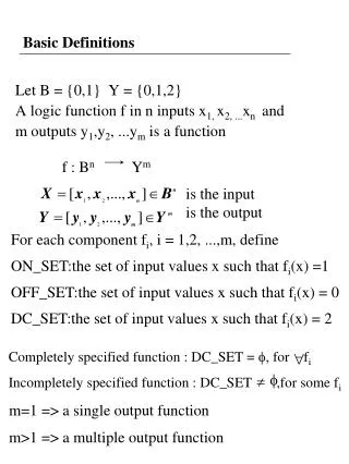
Basic Definitions Let B = {0,1} Y = {0,1,2} A logic function f in n inputs x1, x2, ...xn and m outputs y1,y2, ...ym is a function f : Bn Ym is the input is the output For each component fi, i = 1,2, ...,m, define ON_SET:the set of input values x such that fi(x) =1 OFF_SET:the set of input values x such that fi(x) = 0 DC_SET:the set of input values x such that fi(x) = 2 Completely specified function : DC_SET = f, for fi f Incompletely specified function : DC_SET ,for some fi m=1 => a single output function m>1 => a multiple output function
Representations 1. Truth Table full adder X Y Cin Sum Cout 0 0 0 0 0 0 0 1 1 0 0 1 0 1 0 0 1 1 0 1 1 0 0 1 0 1 0 1 0 1 1 1 0 0 1 1 1 1 1 1 • a multiple output function • Sum : on-set = {(0 0 1), (0 1 0), (1 0 0), (1 1 1)} off-set= {(0 0 0), (0 1 1), (1 0 1), (1 1 0)} • a completely specified function
Representations 2.Geometrical representation 1 variable 0 1 • 2 variables 00 01 10 11 3 variables 011 111 001 101 010 010 110 000 100 sum : on-set ={(0 0 1),(0 1 0),(1 0 0),(1 1 1)} off-set ={(0 1 1),(1 0 1),(1 1 0),(0 0 0)}
Representations 3. Algebraic representations Canonical sum of product Cout = x’yCin + xy’Cin + xyCin’ + xyCin Reduced sum of product Cout = yCin + xCin + xy = yCin + xCin + xyCin’ Multi-level representation Cout = Cin (x + y)+ xy
Representations 4. Reduced Ordered Binary Decision Diagram (ROBDD) Decision graph: f = x1x2 + x3 • Terminal node: • attribute • value (v) = 0 • value (v) = 1 • Non-terminal node: • index (v) = i • two children • low (v) • high (v) • Evaluate an input vector x1 0 1 x2 x2 0 1 1 0 x3 x3 x3 x3 0 0 1 10 1 10 1 0 1 0 1 1 1 0
ROBDD A BDD graph which has a vertex v as root corresponds to the function Fv : (1) If v is a terminal node: a) if value (v) is 1, then Fv = 1 b) if value (v) is 0, then Fv = 0 (2) If F is a nonterminal node(with index(v) = i) Fv(xi , ...xn) = xi’ Flow(v) (xi+1 , ...xn) + xi Fhigh(v) (xi+1 , ...xn)
ROBDD • Reduced BDD : • No distinct vertices v and v’ such that sub- graphs rooted by v and v’ are isomorphism. • No vertex v with low (v) = high (v)
x1 x2 x2 x3 x3 x3 x3 0 1 0 1 0 1 1 1 x1 x2 x2 x3 x3 x3 x3 0 1 x1 x1 x2 x2 x2 x3 x3 0 1 0 1 F=x1x2+x1x3+x1x2x3 0 1 0 1 0 1 0 1 0 1 0 1 0 1 0 1 0 1 0 1 1 1 0 0 0 1 1 0 0 1 1 0 0 1 1 1 0 0 0 1 1 0
ROBDD • Ordered BDD: if x < y, then all nodes representing x precede all nodes representing y • Given an ordering of variables, reduced OBDD is canonical
Example • The size of OBDD depends on the ordering of variables ex : x1x2 + x3x4 x1 < x2 < x3 < x4 x1 1 0 x2 0 1 x3 1 0 x4 0 1 1 0
Example • For a good ordering, the size of an OBDD • remains reasonably small • Multiplier is an exception x1 1 0 x3 x3 1 0 1 0 x2 x2 1 0 1 0 x4 1 0 0 1 x1 < x3 < x2 < x4
Operations on ROBDD Apply f1 <op> f2 (f1, f2 must have the same ordering of variables, then operations can be operated on f1, f2 ) • f1 f2 = (x1’g1 + x1g2)(x1’g3 + x1g4) • = x1’g1g3 + x1g2g4 • = x1’(g1g3) + x1(g2g4) f1 f2 f1 f2 x1 x1 x1 1 1 0 0 0 1 g1 g2 g3 g4 g2g4 g1g3 • f1 + f2 • f1 f2 • etc.
ROBDD 1 f2 : f1’ + f1f2 (implication) • f1 • complement : f • time complexity Reduced O( G log G ) Apply O( G1 G2 )
Property of ROBDD (1) Commonly encountered functions have reasonable representations.(except multiplier) (2) Complementation will not blow up the representation. (3) Canonical form so that equivalence, satisfiability checking can be done easily. (4) Multi-level representation
Representation 5. And-Inverter Graph (AIG) • Simple structure • And-Gates as nodes (shown as circles) with two inputs as edges (shown as arrows) • Inverters edge marked with a dot
Example Ex: y = f( x1,x2,x3) =( (x1 ‧ x2 )’ ‧ (x2 ‧ x3)’)’ = ( x1 ‧ x2 ) + (x2 ‧ x3)
AIG Construction Start from SOP representation Convert to AIG using DeMorgans law x1 + x2 = ( x1 + x2) ’’= ( x1 ’ ‧ x2 ’) ’ 2-input or 3-input and 2-input and 2-input nand
AIG Attributes Size is the number of AND nodes in it Logic level is the number of AND-gates on the longest path from primary input to primary output The inverters are ignored 6 nodes, 4 levels
AIG Canonicity • AIGs are not canonical • ROBDDs are canonical • Same function represented by two functionally equivalent AIGs with different structures • Different structures can still be optimal 6 nodes, 4 levels => area optimal 7 nodes, 3 levels => speed optimal
Characteristic Function Let E be a set and A E The characteristic function A is the function XA : E -> { 0,1 } XA(x) = 1 if x A XA(x) = 0 if x A Ex: E = { 1,2,3,4 } A = { 1,2 } XA(1) = 1 XA(3) = 0 E A
Characteristic Function Given a Boolean function f : Bn -> Bm , the mapping relation denoted as is defined as The characteristic function of a function f is defined for (x,y) s.t. Xf(x,y) = 1 iff (x,y) F
Characteristic Function Ex: y = f( x1,x2 ) = x1 + x2 x1 x2 y 0 0 0 0 1 1 1 0 1 1 1 1 Fy(x1,x2,y) = x1 x2 y F 0 0 0 1 0 0 1 0 0 1 0 0 0 1 1 1 1 0 0 0 1 0 1 1 1 1 0 0 1 1 1 1
Operation on Logic Function • Complement • Intersection • Union • Difference • XOR • F is a tautology • Cofactor • Boolean difference • Consensus operator • Smoothing operator
Cofactor Cofactor operation ( restriction ) cofactor of f with respect to xi=0 cofactor of f with respect to xi=1
Cofator Cofactor with respect to any cube Ex:
Boolean Difference is called Boolean difference of f with respect to x f is sensitive to the value of x when Ex:
Consensus Operator evaluate f to be true for x=1 and x=0 Ex:
Smoothing Operator evaluate f to be true for x=1 or x=0 Ex:
Image Computation by Smoothing Operator • Computation of reachable states of a sequential finite state machine • Given f : Bn -> Bm and let • Use F to obtain the image of a subset A of Bn by f • Compute the projection on Bm of the set F∩(A× Bm) • Smoothing operator and and are used
Example for Image Computation Ex: x1 x2 y z A= {(0, 0), (0, 1)} 0 0 0 0 0 1 1 0 1 0 1 1 1 1 1 1 F(x1, x2, y, z) = x1 x2 y z F 0 0 0 0 1 0 0 0 1 0 0 0 1 0 0 0 0 1 1 0 0 1 0 0 0 0 1 0 1 0 0 1 1 0 1 0 1 1 1 0 1 0 0 0 0 1 0 0 1 0 1 0 1 0 0 1 0 1 1 1 …….
How to build characteristic functions? Ex: x1 x2 y z 0 0 0 0 0 1 1 0 1 0 1 1 1 1 1 1 y = x1+ x2 F1 = z = x1 F2 = F(x1, x2, y, z) = Image computation: S{x1, x2} (F(x1, x2, y, z) )