Download
1 / 61
1.06k likes | 4.42k Vues
The Farmer, Wolf, Duck, Corn Problem. Farmer, Wolf, Goat, Cabbage Farmer, Fox, Chicken, Corn Farmer Dog, Rabbit, Lettuce.

E N D
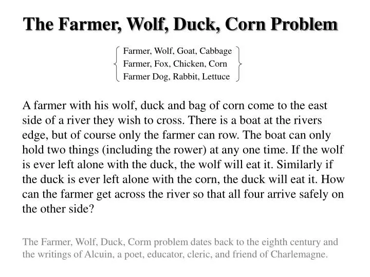
The Farmer, Wolf, Duck, Corn Problem Farmer, Wolf, Goat, Cabbage Farmer, Fox, Chicken, Corn Farmer Dog, Rabbit, Lettuce A farmer with his wolf, duck and bag of corn come to the east side of a river they wish to cross. There is a boat at the rivers edge, but of course only the farmer can row. The boat can only hold two things (including the rower) at any one time. If the wolf is ever left alone with the duck, the wolf will eat it. Similarly if the duck is ever left alone with the corn, the duck will eat it. How can the farmer get across the river so that all four arrive safely on the other side? The Farmer, Wolf, Duck, Corm problem dates back to the eighth century and the writings of Alcuin, a poet, educator, cleric, and friend of Charlemagne.
F W D C F D C W This means that everybody/everything is on the same side of the river. This means that we somehow got the Wolf to the other side.
F F F F F W W W W W D D D D D C C C C C Search Tree for “Farmer, Wolf, Duck, Corn” Illegal State
F F F F F W W W W W D D D D D D C C C C C F F W W D C C Search Tree for “Farmer, Wolf, Duck, Corn” Illegal State Repeated State
F F F F F F F F F F F F F F F F W W W W W W W W W W W W W W W W W W W W D D D D D D D D D D D D D D D D D D D D D C C C C C C C C C C C C C C C C C C C C F F F F F F F F F F F W W W W W W W D D D D D D C C C C C C C Search Tree for “Farmer, Wolf, Duck, Corn” Illegal State Repeated State Goal State
F F F F F F F F F F F F F F F F W W W W W W W W W W W W W W W W D D D D D D D D D D D D D D D D C C C C C C C C C C C C C C C C Initial State Farmer takes duck to left bank Farmer returns alone Farmer takes wolf to left bank Farmer returns with duck Farmer takes corn to left bank Farmer returns alone Farmer takes duck to left bank Success!
Problem Solving using Search • A Problem Space consists of • The current state of the world (initial state) • A description of the actions we can take to transform one state of the world into another (operators). • A description of the desired state of the world (goal state), this could be implicit or explicit. • A solution consists of the goal state*, or a path to the goal state. • * Problems were the path does not matter are known as “constraint satisfaction” problems.
1 2 3 4 5 6 2 1 3 7 8 4 7 6 5 8 Initial State Operators Goal State Slide blank square left. Slide blank square right. …. Move F Move F with W …. FWDC FWDC Distributive property Associative property ... 4 Queens Add a queen such that it does not attack other, previously placed queens. A 4 by 4 chessboard with 4 queens placed on it such that none are attacking each other
Representing the states • A state space should describe • Everything that is needed to solve the problem. • Nothing that is not needed to solve the problem. • For the 8-puzzle • 3 by 3 array • 5, 6, 7 • 8, 4, BLANK • 3, 1, 2 • A vector of length nine • 5,6,7,8,4, BLANK,3,1,2 • A list of facts • Upper_left = 5 • Upper_middle = 6 • Upper_right = 7 • Middle_left = 8 • …. In general, many possible representations are possible, choosing a good representation will make solving the problem much easier. Choose the representation that make the operators easiest to implement.
Operators I 2 1 3 4 7 6 5 8 • Single atomic actions that can transform one state into another. • You must specify an exhaustive list of operators, otherwise the problem may be unsolvable. • Operators consist of • Precondition: Description of any conditions that must be true before using the operator. • Instruction on how the operator changes the state. • In general, for any given state, not all operators are possible. • Examples: • In FWDC, the operator Move_Farmer_Left is not possible if the farmer is already on the left bank. • In this 8-puzzle, • The operator Move_6_down is possible • But the operator Move_7_down is not.
Operators II 2 1 3 4 7 6 5 8 There are often many ways to specify the operators, some will be much easier to implement... Example: For the eight puzzle we could have... • Move 1 left • Move 1 right • Move 1 up • Move 1 down • Move 2 left • Move 2 right • Move 2 up • Move 2 down • Move 3 left • Move 3 right • Move 3 up • Move 3 down • Move 4 left • … • Move Blank left • Move Blank right • Move Blank up • Move Blank down Or
A complete example: The Water Jug Problem A farm hand was sent to a nearby pond to fetch 2 gallons of water. He was given two pails - one 4, the other 3 gallons. How can he measure the requested amount of water? • Two jugs of capacity 4 and 3 units. • It is possible to empty a jug, fill a jug, transfer the content of a jug to the other jug until the former empties or the latter fills. • Task: Produce a jug with 2 units. Abstract away unimportant details • State representation (X , Y) • X is the content of the 4 unit jug. • Y is the content of the 3 unit jug. Define a state representation Define an initial state Initial State (0 , 0) Define an goal state(s) May be a description rather than explicit state Goal State (2 , n) Define all operators • Operators • Fill 3-jug from faucet (a, b) (a, 3) • Fill 4-jug from faucet (a, b) (4, b) • Fill 4-jug from 3-jug (a, b) (a + b, 0) • ...
Once we have defined the problem space (state representation, the initial state, the goal state and operators) are we are done? We start with the initial state and keep using the operators to expand the parent nodes till we find a goal state. …but the search space might be large… …really large… So we need some systematic way to search.
The average number of new nodes we create when expanding a new node is the (effective) branching factor b. • The length of a path to a goal is the depth d. So visiting every the every node in the search tree to depth d will take O(bd) time. Not necessarily O(bd) space. A Generic Search Tree b b2 bd Fringe (Frontier) Set of nonterminal nodes without children I.e nodes waiting to be expanded.
2 1 3 4 7 6 5 8 Branching factors for some problems The eight puzzle has a branching factor of 2.13, so a search tree at depth 20 has about 3.7 million nodes. (note that there only 181,400 different states). Rubik’s cube has a branching factor of 13.34. There are 901,083,404,981,813,616 different states. The average depth of a solution is about 18. The best time for solving the cube in an official championship was 17.04 sec, achieved by Robert Pergl in the 1983 Czechoslovakian Championship. In 1997 the best AI computer programs took weeks (See Korf, UCLA). Chess has a branching factor of about 35, there are about 10120 states (there are about 1079 electrons in the universe).
We are going to consider different techniques to search the problem space, we need to consider what criteria we will use to compare them. • Completeness: Is the technique guaranteed to find an answer (if there is one). • Optimality: Is the technique guaranteed to find the best answer (if there is more than one). (operators can have different costs) • Time Complexity: How long does it take to find a solution. • Space Complexity: How much memory does it take to find a solution.
General (Generic) Search Algorithm function general-search(problem, QUEUEING-FUNCTION) nodes = MAKE-QUEUE(MAKE-NODE(problem.INITIAL-STATE)) loop do if EMPTY(nodes) then return "failure" node = REMOVE-FRONT(nodes) if problem.GOAL-TEST(node.STATE) succeeds then return node nodes = QUEUEING-FUNCTION(nodes, EXPAND(node, problem.OPERATORS)) end A nice fact about this search algorithm is that we can use a single algorithm to do many kinds of search. The only difference is in how the nodes and placed in the queue.
Breadth First SearchEnqueue nodes in FIFO (first-in, first-out) order. Intuition: Expand all nodes at depth i before expanding nodes at depth i + 1 • Complete? Yes. • Optimal? Yes, if path cost is nondecreasing function of depth • Time Complexity: O(bd) • Space Complexity: O(bd), note that every node in the fringe is kept in the queue.
Uniform Cost SearchEnqueue nodes in order of cost 5 2 5 2 5 2 7 1 7 1 5 4 Intuition: Expand the cheapest node. Where the cost is the path cost g(n) • Complete? Yes. • Optimal? Yes, if path cost is nondecreasing function of depth • Time Complexity: O(bd) • Space Complexity: O(bd), note that every node in the fringe keep in the queue. Note that Breadth First search can be seen as a special case of Uniform Cost Search, where the path cost is just the depth.
Depth First SearchEnqueue nodes in LIFO (last-in, first-out) order. Intuition: Expand node at the deepest level (breaking ties left to right) • Complete? No (Yes on finite trees, with no loops). • Optimal? No • Time Complexity: O(bm), where m is the maximum depth. • Space Complexity: O(bm), where m is the maximum depth.
Depth-Limited SearchEnqueue nodes in LIFO (last-in, first-out) order. But limit depth to L L is 2 in this example Intuition: Expand node at the deepest level, but limit depth to L • Complete? Yes if there is a goal state at a depth less than L • Optimal? No • Time Complexity: O(bL), where L is the cutoff. • Space Complexity: O(bL), where L is the cutoff. Picking the right value for L is a difficult, Suppose we chose 7 for FWDC, we will fail to find a solution...
Iterative Deepening Search IDo depth limited search starting a L = 0, keep incrementing L by 1. Intuition: Combine the Optimality and completeness of Breadth first search, with the low space complexity of Depth first search • Complete? Yes • Optimal? Yes • Time Complexity: O(bd), where d is the depth of the solution. • Space Complexity: O(bd), where d is the depth of the solution.
Iterative Deepening Search II Iterative deepening looks wasteful because we reexplore parts of the search space many times... Consider a problem with a branching factor of 10 and a solution at depth 5... 1+10+100+1000+10,000+100,000 = 111,111 1 1+10 1+10+100 1+10+100+1000 1+10+100+1000+10,000 1+10+100+1000+10,000+100,000 = 123,456
Bi-directional Search Intuition: Start searching from both the initial state and the goal state, meet in the middle. • Notes • Not always possible to search backwards • How do we know when the trees meet? • At least one search tree must be retained in memory. • Complete? Yes • Optimal? Yes • Time Complexity: O(bd/2), where d is the depth of the solution. • Space Complexity: O(bd/2), where d is the depth of the solution.
Heuristic Search • The search techniques we have seen so far... • Breadth first search • Uniform cost search • Depth first search • Depth limited search • Iterative Deepening • Bi-directional Search • ...are all too slow for most real world problems uninformed search blind search
7 8 4 3 5 1 6 2 1 2 3 4 5 6 7 8 D FWD FW C C Sometimes we can tell that some states appear better that others...
...we can use this knowledge of the relative merit of states to guide search Heuristic Search (informed search) A Heuristic is a function that, when applied to a state, returns a number that is an estimate of the merit of the state, with respect to the goal. In other words, the heuristic tells us approximately how far the state is from the goal state*. Note we said “approximately”. Heuristics might underestimate or overestimate the merit of a state. But for reasons which we will see, heuristics that only underestimate are very desirable, and are called admissible. *I.e Smaller numbers are better
1 1 2 2 3 3 1 2 3 4 4 5 5 6 6 4 5 6 7 7 8 8 7 8 1 2 3 4 5 6 7 8 N N N N N N N Y Heuristics for 8-puzzle I Current State • The number of misplaced tiles (not including the blank) Goal State In this case, only “8” is misplaced, so the heuristic function evaluates to 1. In other words, the heuristic is telling us, that it thinks a solution might be available in just 1 more move. Notation: h(n) h(current state) = 1
3 1 2 2 8 3 4 4 5 5 6 6 7 7 1 8 Heuristics for 8-puzzle II 3 3 Current State 2 spaces • The Manhattan Distance (not including the blank) 8 3 spaces Goal State 8 1 In this case, only the “3”, “8” and “1” tiles are misplaced, by 2, 3, and 3 squares respectively, so the heuristic function evaluates to 8. In other words, the heuristic is telling us, that it thinks a solution is available in just 8 more moves. 3 spaces 1 Total 8 Notation: h(n) h(current state) = 8
5 6 4 3 4 2 1 3 3 0 2 h(n) We can use heuristics to guide “hill climbing” search. In this example, the Manhattan Distance heuristic helps us quickly find a solution to the 8-puzzle. But “hill climbing has a problem...”
6 1 2 3 4 5 8 6 7 1 2 3 1 2 3 5 7 4 5 8 4 5 6 7 6 7 8 1 2 1 2 3 6 6 4 5 3 4 5 6 7 8 6 7 8 h(n) In this example, hill climbing does not work! All the nodes on the fringe are taking a step “backwards” (local minima) Note that this puzzle is solvable in just 12 more steps.
We have seen two interesting algorithms. • Uniform Cost • Measures the cost to each node. • Is optimal and complete! • Can be very slow. • Hill Climbing • Estimates how far away the goal is. • Is neither optimal nor complete. • Can be very fast. • Can we combine them to create an optimal and complete algorithm that is also very fast?
Uniform Cost SearchEnqueue nodes in order of cost 19 17 19 17 14 16 14 16 13 15 5 2 5 2 5 2 7 1 7 1 5 4 Intuition: Expand the cheapest node. Where the cost is the path cost g(n) Hill Climbing SearchEnqueue nodes in order of estimated distance to goal 17 19 Intuition: Expand the node you think is nearest to goal. Where the estimate of distance to goal is h(n)
The A* Algorithm (“A-Star”)Enqueue nodes in order of estimate cost to goal, f(n) g(n) is the cost to get to a node. h(n) is the estimated distance to the goal. f(n) = g(n) + h(n) We can think of f(n) as the estimated cost of the cheapest solution that goes through node n Note that we can use the general search algorithm we used before. All that we have changed is the queuing strategy. If the heuristic is optimistic, that is to say, it never overestimates the distance to the goal, then… A* is optimal and complete!
Informal proof outline of A* completeness • Assume that every operator has some minimum positive cost, epsilon . • Assume that a goal state exists, therefore some finite set of operators lead to it. • Expanding nodes produces paths whose actual costs increase by at least epsilon each time. Since the algorithm will not terminate until it finds a goal state, it must expand a goal state in finite time. • Informal proof outline of A* optimality • When A* terminates, it has found a goal state • All remaining nodes have an estimate cost to goal (f(n)) greater than or equal to that of goal we have found. • Since the heuristic function was optimistic, the actual cost to goal for these other paths can be no better than the cost of the one we have already found.
How fast is A*? • A* is the fastest search algorithm. That is, for any given heuristic, no algorithm can expand fewer nodes than A*. • How fast is it? Depends of the quality of the heuristic. • If the heuristic is useless (ie h(n) is hardcoded to equal 0 ), the algorithm degenerates to uniform cost. • If the heuristic is perfect, there is no real search, we just march down the tree to the goal. • Generally we are somewhere in between the two situations above. The time taken depends on the quality of the heuristic.
What is A*’s space complexity? A* has worst case O(bd) space complexity, but an iterative deepening version is possible ( IDA* )
A Worked Example: Maze Traversal • Problem: To get from square A3 to square E2, one step at a time, avoiding obstacles (black squares). • Operators: (in order) • go_left(n) • go_down(n) • go_right(n) • each operator costs 1. • Heuristic: Manhattan distance A B C D E 1 2 3 4 5
A3 A A2 A4 B3 B g(A2) = 1 h(A2) = 4 g(B3) = 1 h(B3) = 4 g(A4) = 1 h(A4) = 6 A2 B3 A4 C D E 1 2 3 4 5 • Operators: (in order) • go_left(n) • go_down(n) • go_right(n) • each operator costs 1.
A3 A A4 A1 A2 B3 B g(A2) = 1 h(A2) = 4 g(B3) = 1 h(B3) = 4 g(A4) = 1 h(A4) = 6 A2 B3 A4 C D g(A1) = 2 h(A1) = 5 A1 E 1 2 3 4 5 • Operators: (in order) • go_left(n) • go_down(n) • go_right(n) • each operator costs 1.
A3 A A1 A2 A4 B3 B4 B g(A2) = 1 h(A2) = 4 g(B3) = 1 h(B3) = 4 g(A4) = 1 h(A4) = 6 A2 B3 A4 C3 C D g(A1) = 2 h(A1) = 5 A1 E g(C3) = 2 h(C3) = 3 g(B4) = 2 h(B4) = 5 1 2 3 4 5 C3 B4 • Operators: (in order) • go_left(n) • go_down(n) • go_right(n) • each operator costs 1.
A3 A A1 A2 A4 B3 B4 B1 B g(A2) = 1 h(A2) = 4 g(B3) = 1 h(B3) = 4 g(A4) = 1 h(A4) = 6 A2 B3 A4 C3 C D g(A1) = 2 h(A1) = 5 A1 E g(C3) = 2 h(C3) = 3 g(B4) = 2 h(B4) = 5 1 2 3 4 5 C3 B4 g(B1) = 3 h(B1) = 4 B1 • Operators: (in order) • go_left(n) • go_down(n) • go_right(n) • each operator costs 1.
A3 A A1 A2 A4 B3 B4 B5 B1 B g(A2) = 1 h(A2) = 4 g(B3) = 1 h(B3) = 4 g(A4) = 1 h(A4) = 6 A2 B3 A4 C3 C D g(A1) = 2 h(A1) = 5 A1 E g(C3) = 2 h(C3) = 3 g(B4) = 2 h(B4) = 5 1 2 3 4 5 C3 B4 g(B1) = 3 h(B1) = 4 B1 • Operators: (in order) • go_left(n) • go_down(n) • go_right(n) • each operator costs 1. g(B5) = 3 h(B5) = 6 B5
Optimizing Search(Iterative Improvement Algorithms)I.e Hill climbing, Simulated Annealing Genetic Algorithms • Optimizing search is different to the path finding search we have studied in many ways. • The problems are ones for which exhaustive and heuristic search are NP-hard. • The path is not important (for that reason we typically don’t bother to keep a tree around) (thus we are CPU bound, not memory bound). • Every state is a “solution”. • The search space is (often) continuous. • Usually we abandon hope of finding the best solution, and settle for a very good solution. • The task is usually to find the minimum (or maximum) of a function.
Example Problem I(Continuous) y = f(x) Finding the maximum (minimum) of some function (within a defined range).
Example Problem II(Discrete) The Traveling Salesman Problem (TSP) A salesman spends his time visiting n cities. In one tour he visits each city just once, and finishes up where he started. In what order should he visit them to minimize the distance traveled? There are (n-1)!/2 possible tours.
Example Problem III(Continuous and/or discrete) Function Fitting Depending on the way the problem is setup this, could be continuous and/or discrete. Discrete part Finding the form of the function is it X2or X4or ABS(log(X)) + 75 Continuous part Finding the value for X is it X= 3.1 or X= 3.2
Assume that we can • Represent a state. • Quickly evaluate the quality of a state. • Define operators to change from one state to another. y = log(x) + sin(tan(y-x)) x = 2; y = 7; log(2) + sin(tan(7-2)) = 2.00305 x = add_10_percent(x) y = subtract_10_percent(y) …. A C F K W…..Q A A to C = 234 C to F = 142 … Total 10,231 A C F K W…..Q A A C K F W…..Q A