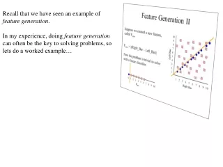
Recall that we have seen an example of feature generation .
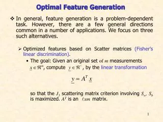
Recall that we have seen an example of feature generation . In my experience, doing feature generation can often be the key to solving problems, so lets do a worked example…. What features can we use classify Japanese names vs Irish names?.


Recall that we have seen an example of feature generation .
E N D
Presentation Transcript
Recall that we have seen an example of feature generation. In my experience, doing feature generation can often be the key to solving problems, so lets do a worked example…
What features can we use classify Japanese names vs Irish names? • The first letter = ‘A’ ? (Boolean feature) Useless Japanese Names Irish Names ABERCROMBIE ABERNETHY ACKART ACKERMAN ACKERS ACKLAND ACTON ADAIR ADLAM ADOLPH AFFLECK AIKO AIMI AINA AIRI AKANE AKEMI AKI AKIKO AKIO AKIRA AMI AOI ARATA ASUKA
What features can we use classify Japanese names vs Irish names? • The first letter = ‘A’ ? (Boolean feature) Useless • The first letter of name Useless (but not useless for Chinese vs Irish, there are very few Irish names that begin with ‘X’, ‘Z’, ‘W’) Japanese Names Irish Names ABERCROMBIE ABERNETHY ACKART ACKERMAN ACKERS ACKLAND ACTON ADAIR ADLAM ADOLPH AFFLECK AIKO AIMI AINA AIRI AKANE AKEMI AKI AKIKO AKIO AKIRA AMI AOI ARATA ASUKA
What features can we use classify Japanese names vs Irish names? • The first letter = ‘A’ ? (Boolean feature) Useless • The first letter of name (Nominal or Ordinal feature) Useless (but not useless for Chinese vs Irish, there are few Irish names that begin with ‘X’, ‘Z’, ‘W’) • The number of letters in the name Slightly useful, Irish names are a litter longer on average. Japanese Names Irish Names ABERCROMBIE ABERNETHY ACKART ACKERMAN ACKERS ACKLAND ACTON ADAIR ADLAM ADOLPH AFFLECK AIKO AIMI AINA AIRI AKANE AKEMI AKI AKIKO AKIO AKIRA AMI AOI ARATA ASUKA
What features can we use classify Japanese names vs Irish names? • The first letter = ‘A’ ? (Boolean feature) Useless • The first letter of name (Nominal or Ordinal feature) Useless (but not useless for Chinese vs Irish, there are few Irish names that begin with ‘X’, ‘Z’, ‘W’) • The number of letters in the name (Ratio feature) Slightly useful, Irish names are a litter longer on average. • The last letter of name Somewhat useful, more Japanese names end in “I” (girls) or “O” (boys), than Irish names do. Japanese Names Irish Names ABERCROMBIE ABERNETHY ACKART ACKERMAN ACKERS ACKLAND ACTON ADAIR ADLAM ADOLPH AFFLECK AIKO AIMI AINA AIRI AKANE AKEMI AKI AKIKO AKIO AKIRA AMI AOI ARATA ASUKA
The number of vowels / world length (Ratio feature) Useful, Japanese names tend to have proportionally more vowels than Irish names. Japanese Names Irish Names ABERCROMBIE 0.45 ABERNETHY 0.33 ACKART 0.33 ACKERMAN 0.375 ACKERS 0.33 ACKLAND 0.28 ACTON 0.33 AIKO 0.75 AIMI 0.75 AINA 0.75 AIRI 0.75 AKANE 0.6 AKEMI 0.6 Vowels = I O U A E
Japanese Names Irish Names ABERCROMBIE 0.45 ABERNETHY 0.33 ACKART 0.33 ACKERMAN 0.375 ACKERS 0.33 ACKLAND 0.28 ACTON 0.33 AIKO 0.75 AIMI 0.75 AINA 0.75 AIRI 0.75 AKANE 0.6 AKEMI 0.6 0 0.5 1.0
Lets do one more. Suppose we want to build a classifier for leaf’s (note that such systems exist) What features should we use? http://leafsnap.com
Can we use size as a feature? Can we use color as a feature? Can we use aspect ratio as a feature? x y Aspect Ratio x/y
This little example of feature generation is something AI researchers spend a lot of time doing. With the right features, most algorithms will work well. Without the right features, no algorithm will work well. There is no single trick that always works, but as we “play” with more and more datasets, we get better at feature generation over time. What feature(s) do we use here?
So far we have only seen features that are real numbers. But features could be: • Boolean (Has Wings?) • Categorical (Green, Brown, Gray) • etc How do we handle such features? The good news is that we can always define some measure of “nearest” for nearest neighbor for basically any kinds of features. Such measures are called distance measures (or sometime, similarity measures).
Let us consider an example that uses Boolean features: • Features: • Has wings? • Has spur on front legs? • Has cone-shaped head? • length(antenna) > 1.5* length(abdomen) • Under this representation, every insect is a just Boolean vector: • Insect17 ={true, true, false, false} • or • Insect17 ={1,1,0,0} • Instead of using the Euclidean distance, we can use the Hamming distance (or one of many other measures). • Which insect is the nearest neighbor of Insect17 ={1,1,0,0}? • Insect1 ={1,1,0,1}, Insect2 ={0,0,0,0}, Insect3 ={0,1,1,1}, Insect3 ={0,1,1,1} • Here we would say Insect17 is in the blue class. Insect17 The Hamming distance between two strings of equal length is the number of positions at which the corresponding symbols are different.
We can use the nearest neighbor algorithm with any distance/similarity function For example, is “Faloutsos” Greek or Irish? We could compare the name “Faloutsos” to a database of names using string edit distance… edit_distance(Faloutsos, Keogh) = 8 edit_distance(Faloutsos, Gunopulos) = 6 Hopefully, the similarity of the name (particularly the suffix) to other Greek names would mean the nearest nearest neighbor is also a Greek name. Specialized distance measures exist for DNA strings, time series, images, graphs, videos, sets, fingerprints etc…
Edit Distance Example Piotr Peter Piero Pedro Pyotr Pierre Pietro Petros How similar are the names “Peter” and “Piotr”? Assume the following cost function Substitution 1 Unit Insertion 1 Unit Deletion 1 Unit D(Peter,Piotr) is 3 It is possible to transform any string Q into string C, using only Substitution, Insertion and Deletion. Assume that each of these operators has a cost associated with it. The similarity between two strings can be defined as the cost of the cheapest transformation from Q to C. Note that for now we have ignored the issue of how we can find this cheapest transformation Peter Piter Pioter Piotr Substitution (i for e) Insertion (o) Deletion (e)
Decision Tree Classifier 10 9 8 7 6 5 4 3 2 1 1 2 3 4 5 6 7 8 9 10 Ross Quinlan Abdomen Length > 7.1? Antenna Length yes no Antenna Length > 6.0? Katydid yes no Katydid Grasshopper Abdomen Length
Decision Tree Classifier 10 9 8 7 6 5 4 3 2 1 1 2 3 4 5 6 7 8 9 10 Here is a different tree. (exercise, draw out the full tree) In general, if we have n Boolean features, the number of trees is: This is both good and bad news. Antenna Length Abdomen Length
Antennae shorter than body? Yes No 3 Tarsi? Grasshopper Yes No Foretiba has ears? Yes No Cricket Decision trees predate computers Katydids Camel Cricket
Decision Tree Classification • Decision tree • A flow-chart-like tree structure • Internal node denotes a test on an attribute • Branch represents an outcome of the test • Leaf nodes represent class labels or class distribution • Decision tree generation consists of two phases • Tree construction • At start, all the training examples are at the root • Partition examples recursively based on selected attributes • Tree pruning • Identify and remove branches that reflect noise or outliers • Use of decision tree: Classifying an unknown sample • Test the attribute values of the sample against the decision tree
How do we construct the decision tree? • Basic algorithm (a greedy algorithm) • Tree is constructed in a top-down recursive divide-and-conquer manner • At start, all the training examples are at the root • Attributes are categorical (if continuous-valued, they can be discretized in advance) • Examples are partitioned recursively based on selected attributes. • Test attributes are selected on the basis of a heuristic or statistical measure (e.g., information gain) • Conditions for stopping partitioning • All samples for a given node belong to the same class • There are no remaining attributes for further partitioning – majority voting is employed for classifying the leaf • There are no samples left
10 9 8 7 6 5 4 3 2 1 1 2 3 4 5 6 7 8 9 10 What should be our Splitting Criteria? Where should I place this line? (or a horizontal line) ????? > ?? Antenna Length yes no Abdomen Length
Information Gain as A Splitting Criteria • Select the attribute with the highest information gain (information gain is the expected reduction in entropy). • Assume there are two classes, P and N • Let the set of examples S contain p elements of class P and n elements of class N • The amount of information, needed to decide if an arbitrary example in S belongs to P or N is defined as 0 log(0) is defined as0
Information Gain in Decision Tree Induction • Assume that using attribute A, a current set will be partitioned into some number of child sets • The encoding information that would be gained by branching on A Note: entropy is at its minimum if the collection of objects is completely uniform
Entropy(4F,5M) = -(4/9)log2(4/9) - (5/9)log2(5/9) = 0.9911 no yes Hair Length <= 5? Let us try splitting on Hair length Entropy(3F,2M) = -(3/5)log2(3/5) - (2/5)log2(2/5) = 0.9710 Entropy(1F,3M) = -(1/4)log2(1/4) - (3/4)log2(3/4) = 0.8113 Gain(Hair Length <= 5) = 0.9911 – (4/9 * 0.8113 + 5/9 * 0.9710 ) = 0.0911
Entropy(4F,5M) = -(4/9)log2(4/9) - (5/9)log2(5/9) = 0.9911 no yes Weight <= 160? Let us try splitting on Weight Entropy(0F,4M) = -(0/4)log2(0/4) - (4/4)log2(4/4) = 0 Entropy(4F,1M) = -(4/5)log2(4/5) - (1/5)log2(1/5) = 0.7219 Gain(Weight <= 160) = 0.9911 – (5/9 * 0.7219 + 4/9 * 0 ) = 0.5900
Entropy(4F,5M) = -(4/9)log2(4/9) - (5/9)log2(5/9) = 0.9911 no yes age <= 40? Let us try splitting on Age Entropy(1F,2M) = -(1/3)log2(1/3) - (2/3)log2(2/3) = 0.9183 Entropy(3F,3M) = -(3/6)log2(3/6) - (3/6)log2(3/6) = 1 Gain(Age <= 40) = 0.9911 – (6/9 * 1 + 3/9 * 0.9183 ) = 0.0183
Of the 3 features we had, Weight was best. But while people who weigh over 160 are perfectly classified (as males), the under 160 people are not perfectly classified… So we simply recurse! no yes Weight <= 160? This time we find that we can split on Hair length, and we are done! no yes Hair Length <= 2?
We need don’t need to keep the data around, just the test conditions. Weight <= 160? yes no How would these people be classified? Hair Length <= 2? Male yes no Male Female
It is trivial to convert Decision Trees to rules… Weight <= 160? yes no Hair Length <= 2? Male no yes Male Female Rules to Classify Males/Females IfWeightgreater than 160, classify as Male Elseif Hair Lengthless than or equal to 2, classify as Male Else classify as Female
Once we have learned the decision tree, we don’t even need a computer! This decision tree is attached to a medical machine, and is designed to help nurses make decisions about what type of doctor to call. Decision tree for a typical shared-care setting applying the system for the diagnosis of prostatic obstructions.
Classification Problem: Fourth Amendment Cases before the Supreme Court I The Fourth Amendment (Amendment IV) to the United States Constitution is the part of the Bill of Rights that prohibits unreasonable searches and seizures and requires any warrant to be judicially sanctioned and supported by probable cause. Suppose we have a 4th Amendment case, Keogh vs. State of California. Keogh argues that the search that found evidence of him taking bribes was and Unreasonable search (U), and the state argues that the search was Reasonable (R). The case is appealed to the Supreme Court, will the court decide U or R? We can use machine learning to try to predict their decision. What should the features be? Keogh vs. State of California = {0,1,1,0,0,0,1,0} • If the search was conducted in a home. • If the search was conducted in a business. • If the search was conducted on one’s person. • If the search was conducted in a car. • If the search was a full search, as opposed to a less extensive intrusion. • If the search was conducted incident to arrest. • If the search was conducted after a lawful arrest. • If an exception to the warrant requirement existed (beyond that of search incident to a lawful arrest). The Statistical Analysis of Judicial Decisions and Legal Rules with Classification Treesjels_1176 202..230 Jonathan P. Kastellec
Classification Problem: Fourth Amendment Cases before the Supreme Court II The Supreme Court’s search and seizure decisions, 1962–1984 terms. Keogh vs. State of California = {0,1,1,0,0,0,1,0} U = Unreasonable R = Reasonable
We can also learn decision trees for individual Supreme Court Members. Using similar decision trees for the other eight justices, these models correctly predicted the majority opinion in 75 percent of the cases, substantially outperforming the experts' 59 percent. Decision Tree for Supreme Court Justice Sandra Day O'Connor
The worked examples we have seen were performed on small datasets. However with small datasets there is a great danger of overfitting the data… When you have few datapoints, there are many possible splitting rules that perfectly classify the data, but will not generalize to future datasets. Yes No Wears green? Male Female For example, the rule “Wears green?” perfectly classifies the data, so does “Mothers name is Jacqueline?”, so does “Has blue shoes”…
Avoid Overfitting in Classification • The generated tree may overfit the training data • Too many branches, some may reflect anomalies due to noise or outliers • Result is in poor accuracy for unseen samples • Two approaches to avoid overfitting • Prepruning: Halt tree construction early—do not split a node if this would result in the goodness measure falling below a threshold • Difficult to choose an appropriate threshold • Postpruning: Remove branches from a “fully grown” tree—get a sequence of progressively pruned trees • Use a set of data different from the training data to decide which is the “best pruned tree”
10 9 8 7 6 5 4 3 2 1 1 2 3 4 5 6 7 8 10 9 How would a DT handle this?
10 9 8 7 6 5 4 3 2 1 1 2 3 4 5 6 7 8 10 9
10 9 8 7 6 5 4 3 2 1 1 2 3 4 5 6 7 8 10 9
10 9 8 7 6 5 4 3 2 1 1 2 3 4 5 6 7 8 10 9
10 9 8 7 6 5 4 3 2 1 1 2 3 4 5 6 7 8 10 9
10 10 100 9 9 90 8 8 80 7 7 70 6 6 60 5 5 50 4 4 40 3 3 30 2 2 20 1 1 10 1 1 2 2 3 3 4 4 5 5 6 6 7 7 8 8 10 10 9 9 10 20 30 40 50 60 70 80 100 90 Which of the “Pigeon Problems” can be solved by a Decision Tree? • Deep Bushy Tree • Useless • Deep Bushy Tree ? The Decision Tree has a hard time with correlated attributes
Advantages/Disadvantages of Decision Trees • Advantages: • Easy to understand (Doctors love them!) • Easy to generate rules • Disadvantages: • May suffer from overfitting. • Classifies by rectangular partitioning (so does not handle correlated features very well). • Can be quite large – pruning is necessary. • Does not handle streaming data easily
Decision Tree Classifier 10 9 8 7 6 5 4 3 2 1 1 2 3 4 5 6 7 8 9 10 Ross Quinlan Abdomen Length > 7.1? Antenna Length yes no Antenna Length > 6.0? Katydid yes no Katydid Grasshopper Abdomen Length
How would we go about building a classifier for projectile points? ?
length I. Location of maximum blade width 1. Proximal quarter 2. Secondmost proximal quarter 3. Secondmost distal quarter 4. Distal quarter II. Base shape 1. Arc-shaped 2. Normal curve 3. Triangular 4. Folsomoid III. Basal indentation ratio 1. No basal indentation 2. 0·90–0·99 (shallow) 3. 0·80–0·89 (deep) IV. Constriction ratio • 1·00 • 0·90–0·99 • 0·80–0·89 4. 0·70–0·79 5. 0·60–0·69 • 0·50–0·59 V. Outer tang angle 1. 93–115 2. 88–92 3. 81–87 4. 66–88 5. 51–65 6. <50 VI. Tang-tip shape 1. Pointed 2. Round 3. Blunt VII. Fluting 1. Absent 2. Present VIII. Length/width ratio 1. 1·00–1·99 2.2·00–2·99 3. 3.00 -3.99 4. 4·00–4·99 5. 5·00–5·99 6. >6. 6·00 width 21225212 length = 3.10 width = 1.45 length /width ratio= 2.13
I. Location of maximum blade width 1. Proximal quarter 2. Secondmost proximal quarter 3. Secondmost distal quarter 4. Distal quarter II. Base shape 1. Arc-shaped 2. Normal curve 3. Triangular 4. Folsomoid III. Basal indentation ratio 1. No basal indentation 2. 0·90–0·99 (shallow) 3. 0·80–0·89 (deep) IV. Constriction ratio • 1·00 • 0·90–0·99 • 0·80–0·89 4. 0·70–0·79 5. 0·60–0·69 • 0·50–0·59 V. Outer tang angle 1. 93–115 2. 88–92 3. 81–87 4. 66–88 5. 51–65 6. <50 VI. Tang-tip shape 1. Pointed 2. Round 3. Blunt VII. Fluting 1. Absent 2. Present VIII. Length/width ratio 1. 1·00–1·99 2.2·00–2·99 3. 3.00 -3.99 4. 4·00–4·99 5. 5·00–5·99 6. >6. 6·00 21225212 Fluting? = TRUE? yes no Base Shape = 4 Late Archaic yes no Length/width ratio = 2 Mississippian
We could also us the Nearest Neighbor Algorithm ? 21225212 21265122 - Late Archaic 14114214 - Transitional Paleo 24225124 - Transitional Paleo 41161212 - Late Archaic 33222214 - Woodland
Avonlea Clovis 1.5 1.0 0.5 11.24 I (Clovis) 0 85.47 II (Avonlea) Shapelet Dictionary 0 100 200 300 400 Arrowhead Decision Tree I II 0 2 1 Clovis Mix Avonlea Decision Tree for Arrowheads It might be better to use the shape directly in the decision tree… Lexiang Ye and Eamonn Keogh (2009) Time Series Shapelets: A New Primitive for Data Mining. SIGKDD 2009 Training data (subset) The shapelet decision tree classifier achieves an accuracy of 80.0%, the accuracy of rotation invariant one-nearest-neighbor classifier is 68.0%.