Chapter 20 Queuing Theory
Chapter 20 Queuing Theory. Description. Each of us has spent a great deal of time waiting in lines. In this chapter, we develop mathematical models for waiting lines, or queues. 8.1 Some Queuing Terminology.

Chapter 20 Queuing Theory
E N D
Presentation Transcript
Description Each of us has spent a great deal of time waiting in lines. In this chapter, we develop mathematical models for waiting lines, or queues.
8.1 Some Queuing Terminology • To describe a queuing system, an input process and an output process must be specified. • Examples of input and output processes are:
The Input or Arrival Process • The input process is usually called the arrival process. • Arrivals are called customers. • We assume that no more than one arrival can occur at a given instant. • If more than one arrival can occur at a given instant, we say that bulk arrivals are allowed. • Models in which arrivals are drawn from a small population are called finite source models. • If a customer arrives but fails to enter the system, we say that the customer has balked.
The Output or Service Process • To describe the output process of a queuing system, we usually specify a probability distribution – the service time distribution – which governs a customer’s service time. • We study two arrangements of servers: servers in parallel and servers in series. • Servers are in parallel if all servers provide the same type of service and a customer needs only pass through one server to complete service. • Servers are in series if a customer must pass through several servers before completing service.
Queue Discipline • The queue discipline describes the method used to determine the order in which customers are served. • The most common queue discipline is the FCFS discipline (first come, first served), in which customers are served in the order of their arrival. • Under the LCFS discipline (last come, first served), the most recent arrivals are the first to enter service. • If the next customer to enter service is randomly chosen from those customers waiting for service it is referred to as the SIRO discipline (service in random order).
Finally we consider priority queuing disciplines. • A priority discipline classifies each arrival into one of several categories. • Each category is then given a priority level, and within each priority level, customers enter service on a FCFS basis. • Another factor that has an important effect on the behavior of a queuing system is the method that customers use to determine which line to join.
8.2 Modeling Arrival and Service Processes • We define ti to be the time at which the ith customer arrives. • In modeling the arrival process we assume that the T’s are independent, continuous random variables described by the random variable A. • The assumption that each interarrival time is governed by the same random variable implies that the distribution of arrivals is independent of the time of day or the day of the week. • This is the assumption of stationary interarrival times.
Stationary interarrival times is often unrealistic, but we may often approximate reality by breaking the time of day into segments. • A negative interarrival time is impossible. This allows us to write • We define1/λ to be the mean or average interarrival time.
We define λ to be the arrival rate, which will have units of arrivals per hour. • An important question is how to choose A to reflect reality and still be computationally tractable. • The most common choice for A is the exponential distribution. • An exponential distribution with parameter λ has a density a(t) = λe-λt. • We can show that the average or mean interarrival time is given by .
Using the fact that var A = E(A2) – E(A)2, we can show that • Lemma 1: If A has an exponential distribution, then for all nonnegative values of t and h,
A density function that satisfies the equation is said to have the no-memory property. • The no-memory property of the exponential distribution is important because it implies that if we want to know the probability distribution of the time until the next arrival, then it does not matter how long it has been since the last arrival.
Relations between Poisson Distribution and Exponential Distribution • If interarrival times are exponential, the probability distribution of the number of arrivals occurring in any time interval of length t is given by the following important theorem. • Theorem 1: Interarrival times are exponential with parameter λ if and only if the number of arrivals to occur in an interval of length t follows the Poisson distribution with parameter λt.
A discrete random variable N has a Poisson distribution with parameter λ if, for n=0,1,2,…, • What assumptions are required for interarrival times to be exponential? Consider the following two assumptions: • Arrivals defined on nonoverlapping time intervals are independent. • For small Δt, the probability of one arrival occurring between times t and t +Δt is λΔt+o(Δt) refers to any quantity satisfying
Theorem 2: If assumption 1 and 2 hold, then Nt follows a Poisson distribution with parameter λt, and interarrival times are exponential with parameter λ; that is, a(t) = λe-λt. • Theorem 2 states that if the arrival rate is stationary, if bulk arrives cannot occur, and if past arrivals do not affect future arrivals, then interarrival times will follow an exponential distribution with parameter λ, and the number of arrivals in any interval of length t is Poisson with parameter λt.
The Erlang Distribution • If interarrival times do not appear to be exponential they are often modeled by an Erlang distribution. • An Erlang distribution is a continuous random variable (call it T) whose density function f(t) is specified by two parameters: a rate parameter R and a shape parameter k (k must be a positive integer). • Given values of R and k, the Erlang density has the following probability density function:
Using integration by parts, we can show that if T is an Erlang distribution with rate parameter R and shape parameter k, • then • The Erlang can be viewed as the sum of independent and identically distributed exponential random variable with rate 1/
Using EXCEL to Computer Poisson and Exponential Probabilities • EXCEL contains functions that facilitate the computation of probabilities concerning the Poisson and Exponential random variable. • The syntax of the Poisson EXCEL function is as follows: • =POISSON(x,Mean,True) gives probability that a Poisson random variable with mean = Mean is less than or equal to x. • =POISSON(x,Mean,False) gives probability that a Poisson random variable with mean =Mean is equal to x.
The syntax of the EXCEL EXPONDIST function is as follows: • =EXPONDIST(x,Lambda,TRUE) gives the probability that an exponential random variable with parameter Lambda assumes a value less than or equal to x. • =EXPONDIST(x,Lambda,FALSE) gives the probability that an exponential random variable with parameter Lambda assumes a value less than or equal to x.
Modeling the Service Process • We assume that the service times of different customers are independent random variables and that each customer’s service time is governed by a random variable S having a density function s(t). • We let 1/µ be the mean service time for a customer. • The variable 1/µ will have units of hours per customer, so µ has units of customers per hour. For this reason, we call µ the service rate. • Unfortunately, actual service times may not be consistent with the no-memory property.
For this reason, we often assume that s(t) is an Erlang distribution with shape parameters k and rate parameter kµ. • In certain situations, interarrival or service times may be modeled as having zero variance; in this case, interarrival or service times are considered to be deterministic. • For example, if interarrival times are deterministic, then each interarrival time will be exactly 1/λ, and if service times are deterministic, each customer’s service time is exactly 1/µ.
The Kendall-Lee Notation for Queuing Systems • Standard notation used to describe many queuing systems. • The notation is used to describe a queuing system in which all arrivals wait in a single line until one of s identical parallel servers is free. Then the first customer in line enters service, and so on. • To describe such a queuing system, Kendall devised the following notation. • Each queuing system is described by six characters: 1/2/3/4/5/6
The first characteristic specifies the nature of the arrival process. The following standard abbreviations are used: M = Interarrival times are independent, identically distributed (iid) and exponentially distributed D = Interarrival times are iid and deterministic Ek = Interarrival times are iid Erlangs with shape parameter k. GI = Interarrival times are iid and governed by some general distribution
The second characteristic specifies the nature of the service times: M = Service times are iid and exponentially distributed D = Service times are iid and deterministic Ek = Service times are iid Erlangs with shape parameter k. G = Service times are iid and governed by some general distribution
The third characteristic is the number of parallel servers. • The fourth characteristic describes the queue discipline: • FCFS = First come, first served • LCFS = Last come, first served • SIRO = Service in random order • GD = General queue discipline • The fifth characteristic specifies the maximum allowable number of customers in the system. • The sixth characteristic gives the size of the population from which customers are drawn.
In many important models 4/5/6 is GD/∞/∞. If this is the case, then 4/5/6 is often omitted. • M/E2/8/FCFS/10/∞ might represent a health clinic with 8 doctors, exponential interarrival times, two-phase Erlang service times, a FCFS queue discipline, and a total capacity of 10 patients.
The Waiting Time Paradox • Suppose the time between the arrival of buses at the student center is exponentially distributed with a mean of 60 minutes. • If we arrive at the student center at a randomly chosen instant, what is the average amount of time that we will have to wait for a bus? • The no-memory property of the exponential distribution implies that no matter how long it has been since the last bus arrived, we would still expect to wait an average of 60 minutes until the next bus arrived.
8.3 Birth-Death Processes • We subsequently use birth-death processes to answer questions about several different types of queuing systems. • We define the number of people present in any queuing system at time t to be the state of the queuing systems at time t. • We call πj the steady state, or equilibrium probability, of state j. • The behavior of Pij(t) before the steady state is reached is called the transient behavior of the queuing system.
A birth-death process is a continuous-time stochastic process for which the system’s state at any time is a nonnegative integer.
Laws of Motion for Birth-Death • Law 1 • With probability λjΔt+o(Δt), a birth occurs between time t and time t+Δt. A birth increases the system state by 1, to j+1. The variable λj is called the birth rate in state j. In most queuing systems, a birth is simply an arrival. • Law 2 • With probability µjΔt+o(Δt), a death occurs between time t and time t +Δt. A death decreases the system state by 1, to j-1. The variable µj is the death rate in state j. In most queuing systems, a death is a service completion. Note that µ0 = 0 must hold, or a negative state could occur. • Law 3 • Births and deaths are independent of each other.
Relation of Exponential Distribution to Birth-Death Processes • Most queuing systems with exponential interarrival times and exponential service times may be modeled as birth-death processes. • More complicated queuing systems with exponential interarrival times and exponential service times may often be modeled as birth-death processes by adding the service rates for occupied servers and adding the arrival rates for different arrival streams.
Derivation of Steady-State Probabilities for Birth-Death Processes • We now show how the πj’s may be determined for an arbitrary birth-death process. • The key role is to relate (for small Δt) Pij(t+Δt) to Pij(t). • The above equations are often called the flow balance equations, or conservation of flow equations, for a birth-death process.
0 1 2 3 4 The “Flow-Balancing Approach” (Entry-Exit Rate Balancing Approach) • In the “rate diagram” given below, think of the following: • Each circle representing a state (i.e., number of customer in the system) has an unknown probability pj, j= 0, 1, 2, … associated with it
We obtain the flow balance equations for a birth-death process:
Solution of Birth-Death Flow Balance Equations • If is finite, we can solve for π0: • It can be shown that if is infinite, then no steady-state distribution exists. • The most common reason for a steady-state failing to exist is that the arrival rate is at least as large as the maximum rate at which customers can be served.
8.4 The M/M/1/GD/∞/∞ Queuing System and the Queuing Formula L=λW • We define . We call p the traffic intensity (utilization) of the queuing system. • We now assume that 0 ≤ p < 1 thusIf p ≥ 1, however, the infinite sum “blows up”. Thus, if p ≥ 1, no steady-state distribution exists.
Derivation of L • Throughout the rest of this section, we assume that p<1, ensuring that a steady-state probability distribution does exist. • The steady state has been reached, the average number of customers in the queuing system (call it L) is given byand
Derivation of Lq • In some circumstances, we are interested in the expected number of people waiting in line (or in the queue). • We denote this number by Lq.
Derivation of Ls • Also of interest is Ls, the expected number of customers in service.
The Queuing Formula L=λW • We define W as the expected time a customer spends in the queuing system, including time in line plus time in service, and Wq as the expected time a customer spends waiting in line. • By using a powerful result known as Little’s queuing formula, W and Wq may be easily computed from L and Lq. • We first define the following quantities L • λ = average number of arrivals entering the system per unit time
L = average number of customers present in the queuing system • Lq = average number of customers waiting in line • Ls = average number of customers in service • W = average time a customer spends in the system • Wq = average time a customer spends in line • Ws = average time a customer spends in service • Theorem 3 – For any queuing system in which a steady-state distribution exists, the following relations hold:L = λWLq = λWqLs = λWs
Example 4 • Suppose that all car owners fill up when their tanks are exactly half full. • At the present time, an average of 7.5 customers per hour arrive at a single-pump gas station. • It takes an average of 4 minutes to service a car. • Assume that interarrival and service times are both exponential. • For the present situation, compute L and W.
Suppose that a gas shortage occurs and panic buying takes place. • To model the phenomenon, suppose that all car owners now purchase gas when their tank are exactly three-fourths full. • Since each car owner is now putting less gas into the tank during each visit to the station, we assume that the average service time has been reduced to 3 1/3 minutes. • How has panic buying affected L and W?
Solutions • We have an M/M/1/GD/∞/∞ system with λ = 7.5 cars per hour and µ = 15 cars per hour. Thus p = 7.5/15 = .50. L = .50/1-.50 = 1, and W = L/λ = 1/7.5 = 0.13 hour. Hence, in this situation, everything is under control, and long lines appear to be unlikely. • We now have an M/M/1/GD/∞/∞ system with λ = 2(7.5) = 15 cars per hour. Now µ = 60/3.333 = 18 cars per hour, and p = 15/18 = 5/6. Then Thus, panic buying has cause long lines.
Problems in which a decision maker must choose between alternative queuing systems are called queuing optimization problems.
More on L = λW • The queuing formula L = λW is very general and can be applied to many situations that do not seem to be queuing problems. • L = average amount of quantity present. • λ = Rate at which quantity arrives at system. • W = average time a unit of quantity spends in system. • Then L = λW or W = L/λ
A Simple Example • Example • Our local MacDonalds’ uses an average of 10,000 pounds of potatoes per week. • The average number of pounds of potatoes on hand is 5000 pounds. • On the average, how long do potatoes stay in the restaurant before being used? • Solution • We are given that L=5000 pounds and λ= 10,000 pounds/week. Therefore W = 5000 pounds/(10,000 pounds/week)=.5 weeks.
A Queueing Model Optimization • Problems in which a decision maker must choose between alternative queueing systems • Example: An average of 10 machinists per hour arrive seeking tools. At present, the tool center is staffed by a clerk who is paid $6 per hour and who takes an average of 5 minutes to handle each request for tools. Since each machinist produces $10 worth of goods per hour, each hour that a machinists spends at the tool center costs the company $10. The company is deciding whether or not it is worthwhile to hire (at $4 per hour) a helper for the clerk. If the helper is hired the clerk will take an average of only 4 minutes to process requirements for tools. Assume that service and arrival times are exponential. Should the helper be hired?
A Queueing Model Optimization • Goal: Minimize the sum of the hourly service cost and expected hourly cost due to the idle times of machinists • Delay cost is the component of cost due to customers waiting in line • Goal: Minimize Expected cost/hour = service cost/hour + expected delay cost/hour • Expected delay cost/hour = (expected delay cost/customer) (expected customers/hour) • Expected delay cost/customer = ($10/machinist-hour)(average hours machinist spends in the system) = 10W • Expected delay cost/hour = 10W • Now compute expected cost/hour if the helper is not hired and also compute the same if the helper is hired

