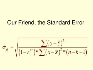
Our Friend, the Standard Error
Our Friend, the Standard Error. What is a Standard Error again?. Think back to the very first day. We were summarizing variables. We wanted to describe dispersion Candy Bar consumption One group consumes {8,5, 6, 7, 9} Mean =7 Another group {2, 4, 12, 7, 10} Mean = 7

Our Friend, the Standard Error
E N D
Presentation Transcript
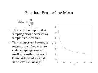
What is a Standard Error again? • Think back to the very first day. We were summarizing variables. • We wanted to describe dispersion • Candy Bar consumption • One group consumes {8,5, 6, 7, 9} Mean =7 • Another group {2, 4, 12, 7, 10} Mean = 7 • Difference is not in mean, difference is dispersion • We define this with mean deviation, variance (s2 / σ2), or standard deviation (s / σ),
Std. Dev. Measures Dispersion Less Dispersion More Dispersion
So we can look at IQ scores σ =15 70 85 μ=100 115 130
Sampling Distribution • What if, instead of looking at the probability of getting at or below a certain level, we took the probability of drawing a sample of 10 people whose average is at or below a certain level? • How will the shape of the distribution change?
Mean IQ scores for samples of 10 people σ = 5 90 95 μ=100 105 110
Sampling Distribution vs. Probability Distribution Sampling Distribution σ = 5 Individual Probability Distribution σ = 15
Sampling Distributions • Sampling Distribution for means • Take a sample of 10, get the mean • Take another sample, get the mean • Repeat samples, what is the distribution of the mean? • Sampling Distribution for difference of means • Take a sample of 10 men, a sample of 10 women, find the difference between their means • Take another sample of 10 men and another sample of 10 women. Find their difference between means • Repeat samples, what is the distribution of the difference between means? • This distribution describes all possible differences for samples of 10 men and 10 women
Sampling Distributions • How should we conceive of the sampling distribution for a regression coefficient, b ? • Take a sample of 50 people and measure their opinion on x and y. Compute b by the formula. • Take another sample of 50 people and measure their opinion on x and y. Compute b again • Repeat samples, calculating b for each one. • Sampling Distribution describes all possible values of b for samples of size 50.
Standard Error of b • Standard Error is the Standard Deviation of a sampling distribution • Recall that for a CI for means, we don’t know where μis, but that we can estimate the standard error, and know that wherever μis, 95% of cases lie within t* standard errors of the mean. • We estimate the std. error and we can use t to create a confidence interval or do a direct hypothesis test
Steps for a Confidence Interval for means • Example: People rate their approval of the Iraq war on a scale from 0-100. We survey 30 people and find a mean of 42 and a std. dev. of 13. Estimate the true approval in the population. • Step 1: Get the information Mean = 42 Std. Dev. = 13 n = 30
Step 2: Estimate the Std. Err. • Step 3: Determine Degrees of Freedom, and choose a value of t* that tells us how far we must go from the mean of the distribution to get 95% of cases • d.f. = 30-1 = 29 • t* = 2.045
Step 4: Plug and Chug • How would you interpret this, both substantively and statistically?
Interpretation • Our estimate is that the mean support score for the Iraq war is 42 + 4.93 • In repeated samples of the same size from the same population, 95% of all samples would yield an interval that contains the true population mean. • While it is possible that our sample is one of the few that doesn’t contain the true mean, it is most likely that it does contain it.
Same logic applies to Regression • Step 1: Get your information • Run your regression (in Stata or by hand) • Find sample regression coefficient (b) and estimated root mean square error from regression
Step 2: Estimate Standard Error • For 1 independent variable, • Let’s talk about this for a minute • What is σε2 ? Have we seen it before? • Sum of Squared Errors (RSS) • We don’t know it, but RMSE is our estimate,
Step 3: Determine Degrees of Freedom • d.f. = n – k – 1 • Choose an appropriate value of t from the table.
Step 4: Calculate the C.I. • What do we know about the samp. distrib. of b? • We do not know the true value of β • We know something about the shape of the distribution * If the 10 assumptions hold it is distributed t with n-k-1 degrees of freedom, with β as its mean. • We still don’t know β, but wherever it is, 95% possible sample b’s are within t* standard deviations • If 95% of sample b’s are within t* std. devs. of the mean, than we can make an interval around our b and this strategy will, 95 times out of 100, yield an interval that contains the true population b.
What do we Know Now ? • If we took repeated samples, 95% would yield an interval that contains the true β • If our interval does not contain 0, we are 95% confident that β≠ 0 (but it could be that our interval doesn’t contain β and that β=0, so there is still 5% risk) • If our interval does contain 0, we cannot be sure that β≠ 0. So, we say our value of b is not statistically significant (we fail to reject the null that β=0)
Example (by hand) • We want to predict someone’s FT score for Bush in 2000 by knowing how the feel about Gore. We sample 50 people • What is D.V., I.V. ? • We find b = -.82, RMSE = 2.518
Example (by hand) • Step 3: Get t stuff • d.f. = n-k-1 = 50-1-1=48 • t*=2.021 • Step 4: Plug and Chug • CI for b is (-.98, -.65). In repeated samples, 95% of CI’s would contain β
In Stata . regress bushft goreft Source | SS df MS Number of obs = 50 -------------+--------------------------- F( 1, 48) = 96.83 Model | 26535.5757 1 2735.4457 Prob > F = 0.0000 Residual | 25531.2593 48 1403.3364 R-squared = 0.6686 -------------+--------------------------- Adj R-squared = 0.6617 Total | 43937.38 49 896.681224 Root MSE = 2.518 ------------------------------------------------------------------------- bushft | Coef. Std. Err. t P>|t| [95% Conf. Interval] -----------+------------------------------------------------------------- goreft | -.8194653 .0832774 -9.84 0.000 -.9869057 -.6520249 _cons | 95.43093 5.42934 17.58 0.000 84.51451 106.3474 ------------------------------------------------------------------------- Confidence Interval for b does not contain 0, it is significant Confidence Interval for a does not contain 0, it is significant
If We had seen … . regress bushft perotft Source | SS df MS Number of obs = 50 -------------+--------------------------- F( 1, 48) = 12.83 Model | 29375.4547 1 29375.4547 Prob > F = 0.0434 Residual | 14561.9253 48 303.373444 R-squared = 0.1263 -------------+--------------------------- Adj R-squared = 0.0127 Total | 43937.38 49 896.681224 Root MSE = 27.418 ------------------------------------------------------------------------- bushft | Coef. Std. Err. t P>|t| [95% Conf. Interval] -----------+------------------------------------------------------------- perotft | -.3922048 .24779 -1.58 0.000 -.9869057 .2024961 _cons | 51.43093 5.42934 12.58 0.000 36.51451 65.3474 ------------------------------------------------------------------------- Confidence Interval for b contains 0, it is not significant Confidence Interval for a does not contain 0, it is significant
Practice: • To highlight the way this works, let’s show that we can work backwards. • Can we figure out the standard error? . regress bushft goreft Source | SS df MS Number of obs = 50 -------------+--------------------------- F( 1, 48) = 96.83 Model | 26535.5757 1 2735.4457 Prob > F = 0.0000 Residual | 25531.2593 48 1403.3364 R-squared = 0.6686 -------------+--------------------------- Adj R-squared = 0.6617 Total | 43937.38 49 896.681224 Root MSE = 2.518 ------------------------------------------------------------------------- bushft | Coef. Std. Err. t P>|t| [95% Conf. Interval] -----------+------------------------------------------------------------- goreft | -.8194653 .0832774 -9.84 0.000 -.9869057 -.6520249 _cons | 95.43093 5.42934 17.58 0.000 84.51451 106.3474 ------------------------------------------------------------------------- ?
Yes! • Formula for Confidence interval: • Fill in what we know
C.I. for Multiple Regression • Two differences • Each coefficient (b1, b2, b3,… bn) has its own sampling distribution, so each one has its own standard error. Each one could take on a totally different range of values with changes in samples • Formula for Std. Error Changes
One last trick • Stata automatically gives 95% C.I. What if you want 99% C.I.s? • Remember the formula? Only adjustment is in your choice of t*. You can go back and do this by hand, using b + t*(S.E.), just choosing t* from the 99% column • Alternatively, tell Stata you want 99% regress y x1 x2 x3, level(99)
What you should know and be able to do: • Interpret the Confidence Intervals in Stata output. Do this for all intervals (not just 95%) • Calculate C.I.’s for any level of risk by hand given the formulas and necessary information • Do both of these in both bivariate and multiple regression settings • Work backwards through this, given necessary information
Direct Hypothesis Testing with Regression Coefficients • Recall that when we wanted to see a difference between two means, we could either to C.I. approach or Hypo Test • If we assume the real difference is “0” in the population, we can calculate a t score an assess the chances of getting a difference this big by sampling error alone.
A random sample of 16 governments from European countries with parliamentary systems finds an average government length of 3.4 years with a standard deviation of 1.2 years. 11 randomly sampled Non-European countries with parliamentary systems had an average government duration of 2.7 years with a standard deviation of 1.5 years. • Test the hypothesis that European Governments and Non-European governments differ in average duration.
Hypo Test: Steps • State the null and alternative hypothesis -Null: No Difference Between Euro gov’ts and non-Euro gvts. -Alternative: European and non-European gov’ts are different • Compute the standard error for the sampling distribution for difference of means n2 = 11 x2 = 2.7 S2 = 1.5 n1 = 16 x1 = 3.4 S1 = 1.2
With a Direct Hypothesis Test 3. Get an appropriate t value from the t table (2.060, for 25 d.f. ). 4. Compute the t score for your difference
Conclusion • Step 5: The t-score we computed (1.29) is less than the critical t from the table (2.060), so we fail to reject the null hypothesis In repeated samples of these sizes from the same population, more than 5% of samples would show a difference this big by sampling error alone
By the Pictures -2.060 +2.060 1.29 0 Hypothesis Test Units of Standard Deviation
Hypothesis Testing with Regression Coefficients • Step 1: State Hypothesis • Null: β = 0 (No relationship between x and y) • Alternative: β≠ 0 (Some relationship) • Step 2: Compute the Standard Error of the sampling distribution for b
Hypo Test Steps • Step 3: Choose critical t (t*) from the table • Recall that if Σe2 is normally distributed, we can use the t distribution with n-k-1 degrees of freedom • This gives us the range in which 95% of values b could take on by random chance (given our sample size) if the true population regression coefficient is zero
Hypo Test Steps • Step 4: Compute t score for your data • Step 5: If your t-score is greater than the critical value, t*, from the table, we reject the null hypothesis. If your t score is less than the critical value, we fail to reject the null hypothesis
Example: • Regression using a sample of size 50 yields the following equation: ADA Score = 5.04 + RegDems*.00047 • Std. Err. for a=1.45, for b=.00018 • Step 1: State Nulls • Step 2: Standard Errors given • Step 3: Choose t* = 2.021
Example • Step 4: Calculate t from your data • Step 5: For a, t > t*, so we reject the null hypothesis (it is “significant”). For b, t >t*, so we again reject the null (it is also “statistically significant”).
Review Confidence Levels • We are used to setting α (level of risk) at .05. This gives a 95% level of confidence • We have also switched to 99% or 90% levels of confidence (α =.01 or .1, respectively) • What are the tradeoffs involved? • Said another way, α represents Type I Error, while (1- α) represents Type II Error
New Concept: p values • Some regression coefficients might be “significant” (we reject the null) at the 95% confidence level (α = .05), but not significant at the 99% level. • Others might be significant at the 99.99% level but we don’t realize it if we only look at the 95% level • What if we could know the “exact” smallest level of α at which we still reject the null • i.e., We reject at 95%, we fail to reject at 99%, we could search and find that it is significant at 97.4% level (α=2.6), but not at 97.5% (α=2.5)
How is this done? • Doing this many confidence intervals by hand would ultimately be painful • Remember, though that • So we can just go to the t-table and scan across the columns, and see what the best we can do is. Of course, we only have .20, .10, .05, .025, .01, and .001 on our tables, so we cannot be terribly precise • Suppose t = 2.87, two-tailed. Assume 13 d.f.
t=2.87 • So our p value is less than .02, but more than .01
How is this done? • Stata does it automatically and with precision. • If this column < .05, we reject the null . regress turnout diplomau mdnincm Source | SS df MS Number of obs = 426 ---------+------------------------------ F( 2, 423) = 31.37 Model | 1.4313e+11 2 7.1565e+10 Prob > F = 0.0000 Residual | 9.6512e+11 423 2.2816e+09 R-squared = 0.1291 ---------+------------------------------ Adj R-squared = 0.1250 Total | 1.1082e+12 425 2.6076e+09 Root MSE = 47766 -------------------------------------------------------------------- turnout | Coef. Std. Err. t P>|t| [95% Conf. Interval] ---------+---------------------------------------------------------- diplomau | 1101.359 504.4476 2.18 0.030 109.823 2092.895 mdnincm | 1.111589 .4325834 2.65 0.009 .261308 1.961869 _cons | 154154.4 9641.523 15.99 0.000 135203.1 173105.6 --------------------------------------------------------------------
Substantive significance • A variable may be “statistically significant” at the .05 level (95% confidence level) • This does not mean this variable is very important. The coefficient could be significant but very small. • Example: States try to reduce high school class sizes to improve the quality of education • We find these results:
Dep. Var.: Index for educational quality ranging from 0-100 • Interpret Class Size • Statistically Significant • Substantively …? • Interpret Spending • Statistically Significant • Substantively Sig. • Interpret Med. Income • Not Statistically Sig. • Constant • Statistically Sig. • No independent interp.
What you should know and be able to do: • Execute a hypothesis test for the significance of regression coefficients by hand given b and the standard error of b (or a and the standard error of a) • Interpret the results of a “by-hand” hypothesis test • Interpret the hypothesis-test output in Stata, including t-scores and p-values • Explain what the standard error of b means • Explain hypothesis tests from the standpoint of repeated samples • Evaluate substantive Significance
Old trick for a new dog • We did one-tailed tests for difference of means when we knew that one group would be greater than the other • If we know that there is a positive relationship between x and y (b > 0), we can specify a one-tailed test • Same holds for knowing that there is a negative relationship (b < 0)
Guidelines for 1-tailed test • You must specify 1-tailed before you type regress • Stata doesn’t do 1-tailed tests • You must convert Stata’s two-tailed test into a one-tailed test • Take the reported p-value (not the t-value!) and divide by two to get the one-tailed p-value (then compare that to .05 or .01 or whatever)
Example • Stata reports a p-value for education of .03 If we divide by two, the one-tailed p-value is .015 • The most important difference will be for values between .10 and .05 (they become sig. at .05-.25 level) . regress turnout diplomau mdnincm Source | SS df MS Number of obs = 426 ---------+------------------------------ F( 2, 423) = 31.37 Model | 1.4313e+11 2 7.1565e+10 Prob > F = 0.0000 Residual | 9.6512e+11 423 2.2816e+09 R-squared = 0.1291 ---------+------------------------------ Adj R-squared = 0.1250 Total | 1.1082e+12 425 2.6076e+09 Root MSE = 47766 -------------------------------------------------------------------- turnout | Coef. Std. Err. t P>|t| [95% Conf. Interval] ---------+---------------------------------------------------------- diplomau | 1101.359 504.4476 2.18 0.030 109.823 2092.895 mdnincm | 1.111589 .4325834 2.65 0.009 .261308 1.961869 _cons | 154154.4 9641.523 15.99 0.000 135203.1 173105.6 --------------------------------------------------------------------