PanSTARRS Gigapixel Camera System
650 likes | 1.07k Vues
PanSTARRS Gigapixel Camera System. John Tonry (IFA), Gerard Luppino (IFA), Peter Onaka (IFA), Barry Burke (MITLL). Scope of Gigapixel Camera effort. WIYN telescope collaboration. OTA development status OTA test plan OTA package, focal plane and cryostat design.

PanSTARRS Gigapixel Camera System
E N D
Presentation Transcript
PanSTARRS Gigapixel Camera System John Tonry (IFA), Gerard Luppino (IFA), Peter Onaka (IFA), Barry Burke (MITLL) • Scope of Gigapixel Camera effort. • WIYN telescope collaboration. • OTA development status • OTA test plan • OTA package, focal plane and cryostat design. • OTA controller electronics design and development. Outline
Scope of Gigapixel Camera Effort Part of Detector/Camera System Scope?
WIYN Telescope Collaboration • Non Binding Collaboration • WIYN Developing One-Degree Imager (ODI) • Camera System Nearly Identical to one of the PanSTARRS Gigapixel Cameras.
Outline • Overview of OTA • Principal design and process challenges • Pixel layout • Logic design, fabrication, and recent results • Metallization and interconnects • Other OTA design issues and options • Die size and pads • Enhanced substrate E fields • Compatibility of design with CMOS option • Mini-OTA (MOTA) options • Process options and lot-1 splits • Design status and summary
Orthogonal Transfer Array (OTA) OTCCD cells • 88 array of small OTCCDs , each ~500 500 pixels* • OTCCD cells independently clocked via on-chip control logic • Cells read out one row at a time at 1-MHz read rate; readout time ~ 2 s • Subset of cells (typically five) selectable for tracking guidestars at ~30-Hz rates *(12 um: 480 x 496; gaps 9 x 28, 10 um: 574 x 594; gaps 11 x 35)
DetectorDetails – Overview Each CCD cell of a 4K 4K OTA • Independent ~500 500-pixel CCDs • Individual or collective addressing • 1 arcmin field of view • Dead cells excised, yield >50% • Bad columns confined to cells • Cells with bright stars for guiding • 8 output channels per OTA • Fast readout (8 amps, 2 sec) • Disadvantage – 0.1 mm gaps, but gaps and dead cells are dithered out anyway 5 cm
Outline • Overview of OTA • Principal design and process challenges • Pixel layout • Logic design, fabrication, and recent results • Metallization and interconnects • Other OTA design issues and options • Die size and pads • Enhanced substrate E fields • Compatibility of design with CMOS option • Mini-OTA (MOTA) options • Process options and lot-1 splits • Design status and summary
Principal Challenges • OTCCD • OTCCD yield was low until recently (lot 4) • Pixel layout appears to be critical to high yield • Control logic • Except for some preliminary test structures nMOS has not been part of Lincoln CCD process • Design and simulation learning curve • Metallization • Extensive use of two levels of metal • New planarized metal process recently developed on other programs; test-structure data are encouraging
OTCCD Process Issues • Polysilicon stackup must be minimized • High stresses may be a factor • Metallization process requires low gate profile (see subsequent chart) • OTCCD lot 4 had high yield after pixel re-design • Design rules • Max of two poly layers over channel stops • Max of three poly layers over channel regions
Poly Pileup Areas of three- and four-poly stacks Three-poly stacks only Revised pixel layout Original pixel layout
OTCCD Types • Type 1 OTCCD • Most experience with this style: 2K 4K, 1024 1320, 512 512 (all 15-µm pixels) • 2K 4K now has good yield (CCID-28, lot 4) • Type 2 • Higher symmetry but no obvious fabrication advantage • Only 512 512 (15-µm pixels) made thus far
Poly stackup Minimum poly linewidth Well capacity OTA Pixel Designs • Experience to date is with 15-µm pixels • Desired pixel sizes are ≤ 12 µm • 12-µm pixel: low risk • 10 µm: moderate risk • 8 µm: high risk • Tight trade space: Poly1, poly2 layout Channel stops Poly3, poly4 layout Example of 10-µm pixel design
Pixel Design Choices • Current plan: four versions of OTA, each with different pixel layout • Two 12-µm-pixel designs as lowest risk • OTA-a: type 1 • OTA-b: type 2 • Two 10-µm pixel designs, both scaled from 12-µm layouts, as somewhat higher risk but closer to desired pixel size • OTA-c: type 1 (scaled OTA-a pixel) • OTA-d: type 2 (scaled OTA-b pixel) Pixel a Pixel b
Logic Design Considerations • Requirements • Cells must be independently addressable • Parallel clocks for each cell can be set to one of three states • Active (image readout, update pixel shifts, etc.) • Standby (image acquisition between updates) • Floating (shorted phases) • Cell outputs read out one row at a time • Maximum of one cell/column read at any time • Desired • Low FET count, compact layout • Low power • Compatible with parallel shift rate > 100 kHz
Control Logic Overview • NMOS logic chosen • Easy to add to n-channel CCD process(+) • Power inefficient (-) • Early start on development • Oct 2002: SPICE parameter extraction from test MOSFETs on CCID-28, lot 4 • February 2003: preliminary OTA logic designs added to SST mask set • June 2003: logic designs on SST wafers in test!
Addressing and Control Logic:Current Design • Data are latched at each cell until addressed again • Flexible operation • Cell can be clocked with video on or off • Standby mode during science image acquisition • Defective parallel gates can float
Final Control Logic Design • 39 FETs, 0.6–0.8 mW power dissipation • Operation with VDD=5.0 V; accepts inputs with 5-V CMOS-compatible levels • Further variants under study for inclusion as test structures
Logic Designs on SST Wafers • Designs • Simple building-block circuits • Preliminary OTA addressing and control logic (since modified) • Advanced aggressive designs • Important validation of design and simulation methodologies Original OTA logic design (61 FETs) Closeup of circuit
Q Q First Test Circuit Results • Latch circuit works for VDD= 5.0 V • Two versions (different design rules) successful • Threshold voltages somewhat higher than expected • Fix is simple implant-dose adjustment D Q CLK D CLK
Additional NMOS Test Results • First version of OTA control logic works! • Design from January; uses 61 FETs • Functions with VDD=5 V
Metallization • OTA uses large amount of wiring • Two levels of metal (light and dark blue) • Design rules kept deliberately relaxed • Line widths and spacings 5 µm
Metallization Process: Planarized Dielectrics with W Plugs • Same approach as used in current CMOS processes • Process outline: • Thick oxide deposited and planarized (CMP) • Contact holes etched, filled with W (damascene process) • Metal straps • Repeat for second metal • Advantages • W plugs can be narrower and deeper than conventional contacts for AlSi • Planar surface better for fine lithography • Shorts yield from test wafers is high • Poly stackups must be minimized to maintain poly/metal isolation Cross section from CCID-34 test wafer
Metal Strapping Experiments • Used existing large imager (~20 cm2) mask set and added metal straps over chanstops • Critical test (gate shorts induced by straps) showed high yield • Significant differences from standard LL CCD process • Dry-etched metal (vs. wet) • Ti/TiN/AlSi (vs. AlSi) • W plugs (new) Metal straps
Metallization Options • Placing digital-related lines over pixel arrays increases fill factor by 3.3% • Is this a worthwhile gain? • Process implications • Greater chance of metal/poly shorts • More room for metal lines: fewer metal/metal shorts • Metal lines can be wider: faster clocking, less vulnerable to line breaks • Metal-over-pixels option requires three mask changes
Outline • Overview of OTA • Principal design and process challenges • Pixel layout • Logic design, fabrication, and recent results • Metallization and interconnects • Other OTA design issues and options • Die size and pads • Enhanced substrate E fields • Compatibility of design with CMOS option • Mini-OTA (MOTA) options • Process options and lot-1 splits • Design status and summary
Die Size • Exclusion zone > 5 mm chosen die size = 49.5 49.5 mm • Compatible with STA/Dalsa requirements • Saw kerf ≈ 70 µm sawn die size = 49.43 49.43 mm
Pad Layout • Mirror symmetric pad layout: FI and BI devices use same package and I/O Center Right side Left side
Deep Depletion with Substrate Bias • Chanstop and bottom substrate electrically connected: bottom substrate cannot be biased • Chanstop and bottom substrate electrically isolated: bottom substrate can be biased
Advantages of Deep Depletion Vsub Vsub Front-illuminated – Improved high-energy x-ray response Back illuminated – Increased vertical E fields tighter PSF
Measured Depletion Depths • Deep-depletion CCD (CCID-42) • 512512, 15-µm-pixel frame-transfer device • Same pinouts as all previous 5122 devices • Data taken from capacitance-voltage test structure that represents CCD layout • Depletion depths > 150 µm easily achieved
X-ray Data from MIT/CSR • Si absorption length at 22 keV=1370 µm • QE depletion depth • Improved detection of high-quality events • ~2 count increase consistent with ~2 increase in depletion depth
Deep Depletion • Current plans • Thin four CCID-42 chips to varying thicknesses (60 – 150 µm) • Measure QE and PSF vs. thickness and substrate bias (data relevant to Pan-STARRS) • Devices ready for test in 2 – 3 months • Backside treatment: II/LA or chemisorption charging? • OTA design can include deep-depletion option
Why OTA/CMOS Hybrid? • Advantages • Risk reduction if monolithic OTA fails • Simplifies OTCCD processing (no NMOS, large network of metal lines) • Pathfinder for more on-sensor processing in CMOS • Possible improvement in fill factor • Disadvantages • Additional costs: CMOS design, fab & test, bump bonding • Adjustments to thinning process
Hybrid OTA OTA chip CMOS control chip Bump bonding Hybrid OTA/CMOS sensor
OTA Design for CMOS Hybrid • Optional metal mask brings all OTA cell functions to pads for bumping • Can be done as process split (one mask change, two mask steps deleted) • Fill factor uncertain; better than baseline but maybe not as good as metal-over-pixels • Space allows double pads/function for redundancy OTA cell
CMOS/OTA Attachment 3. Attach handle wafer (with epoxy) 4. Flush-thin CCD wafer 1. Attach CMOS die to OTA wafer 2. Underfill with epoxy
OTA/CMOS Hybrid Sensor After CCD thinning, pad-via etch, back-surface treatment After bonding
Mini OTAs • MOTA is 22-cell version of OTA • Opportunity to try advanced features • Two-phase serial register • Dual output gates • Higher performance logic designs • Useful as monitor devices (QE, PSF, etc.) • ~12 die possible • Fits in conventional PGA Tentative wafer layout
12m 12m Type 1 Type 2 10m 10m Type 1 Type 2 Process Splits for Lot 1
Test Plan for OTAs • Device selection phase (Mar –Jun 2004) • Approximately 16 different devices • Pixel size, CMOS logic, deeper depletion, shutter, etc. • MOTAs with more exotic choices • Serious, thorough testing necessary during a short time which will lead to final, production OTA design choices. • Production testing (Oct 2004 – Oct 2006) • Wafer probe frontside for S/O (powered up?); excise cells? • Wafer probe backside, cold (packages are valuable) • OTA test, tune, and select • 300 OTAs need testing (20,000 CCDs!), so we need well designed, stable test setups, software, and analysis tools.
Design Selection Phase • Clocking / pixel performance • CTI • Pocket density • Cosmetics • Dark current • Image persistence • QE non-uniformity, fringing • QE • Full well • Clocking time constants • Charge diffusion • Goodies • Electronic shutter • 2-phase serial
Design Selection Phase • Amplifier performance • Read noise • 1/f knee – noise versus speed • Linearity • Amplifier / logic glow • Cross – talk: inter-cell, inter-OTA • Goodies: • pJFET?
Design Selection Phase • Package/cells • CR and radioactivity rate • Addressing • Cell excision: • Laser/ultrasonic excision? • Tri-state logic? • OTA metrology • Flatness • Placement of dice on package • Epoxy squeeze-out, epoxy voids • Bond wire masking / covering of bright scatterers
Hardware • Controller • New controllers must be thoroughly tested and understood! • Features • Alter clocking / bias voltages • Read out full chip or arbitrary binned subarray • 1 Mpix readout at 4e- noise • Slow readout for better noise • Dewars and focal planes • 1 OTA, quick swap • 2 x 4 OTA, 2 controller: test 2x2, QUOTA/OCTOTA for sky • MOTA package / testing • Test setup • X-ray source • Monochromator / photodiode (inside dewar?) • Optical images focussed on detectors (sub pixel?)
Testing Setup • Replace normal dewar window with “Snoutus Maximus” • Simultaneous x-ray stimulation from Fe55 or optical light • Complete test sequence in one 5 hour cool-down cycle
X-ray Testing - Quantitative Parallel CTI Pixel Value Pixel Value Row Row Serial CTI Column Column Perfect CTE Bad CTE
X-ray Testing - Quantitative • Slop2 • Determine and subtract bias level • Generate and subtract “local sky” • Reconstruct split pixels (if requested) • Identify K-alpha pixel values as a function of (x,y) • Fit a plane • Gain derived from plane intercept at (0,0) • Noise derived from overclocks • CTE parallel from y slope, CTE serial from x slope • Other features sometimes visible in pixel value plots
X-ray Testing - Quantitative • Plot pixel values as a function of column (x) and row (y) • K-alpha (1620 e-) and K-beta (1780 e-) are visible • Junk on right comes from a bright defect and associated bleed column.
X-ray Testing - Quantitative • Here’s the associated histogram of pixel values. K K