A Fast and Scalable Nearest Neighbor Based Classification
A Fast and Scalable Nearest Neighbor Based Classification. Taufik Abidin and William Perrizo Department of Computer Science North Dakota State University. Outline. Nearest Neighbors Classification Problems

A Fast and Scalable Nearest Neighbor Based Classification
E N D
Presentation Transcript
A Fast and Scalable Nearest Neighbor Based Classification Taufik Abidin and William Perrizo Department of Computer Science North Dakota State University
Outline • Nearest Neighbors Classification • Problems • SMART TV (SMall Absolute diffeRence of ToTal Variation): A Fast and Scalable Nearest Neighbors Classification Algorithm • SMART TV in Image Classification
Unclassified Object Search for the K-Nearest Neighbors Vote the class Training Set Classification Given a (large) TRAINING SET, R(A1,…,An, C), with C=CLASSES and (A1…An)=FEATURES Classification task is: to label the unclassified objects based on the pre-defined class labels of objects in the training set Prominent classification algorithms: SVM, KNN, Bayesian, etc.
Can we make it faster and scalable? Problems with KNN • Finding k-nearest neighbors is expensive when the training set contains millions of objects (very large training set) • The classification time is linear to the size of the training set
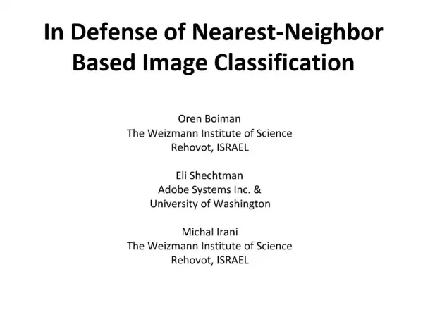
R[A1] R[A2] R[A3] R[A4] R A1 A2 A3 A4 010 111 110 001 011 111 110 000 010 110 101 001 010 111 101 111 101 010 001 100 010 010 001 101 111 000 001 100 111 000 001 100 010 111 110 001 011 111 110 000 010 110 101 001 010 111 101 111 101 010 001 100 010 010 001 101 111 000 001 100 111 000 001 100 2 7 6 1 6 7 6 0 2 7 5 1 2 7 5 7 5 2 1 4 2 2 1 5 7 0 1 4 7 0 1 4 0 1 0 1 1 1 1 1 0 0 0 1 0 1 1 1 1 1 1 1 0 0 0 0 0 1 0 1 1 0 1 0 1 0 0 1 0 1 0 1 1 1 1 0 1 1 1 1 1 0 1 0 1 0 0 0 1 1 0 0 0 1 0 0 1 0 0 0 1 1 0 1 1 1 1 0 0 0 0 0 1 1 0 0 1 1 1 0 0 0 0 0 1 1 0 0 0 1 0 1 0 0 0 0 1 0 01 0 1 0 0 1 01 P11 P12 P13 P21 P22 P23 P31 P32 P33 P41 P42 P43 0 0 0 0 1 01 0 0 0 0 1 0 0 10 01 0 0 0 1 0 0 0 0 0 0 0 1 01 10 0 0 0 0 1 10 0 1 0 0 0 1 0 1 ^ ^ ^ ^ ^ ^ ^ ^ ^ 0 0 1 0 1 01 0 1 0 P-Tree Vertical Data Structure = R11 R12 R13 R21 R22 R23 R31 R32 R33 R41 R42 R43 The construction steps of P-trees: 1. Convert the data into binary 2. Vertically project each attribute 3. Vertically project each bit position 4. Compress each bit slice into a P-tree
TV g TV(X,)=TV(X,x33) 1 1 2 2 a 3 3 4 4 5 5 a- X Total Variation The Total Variation of a set X about (the mean), , measures total squared separation of objects in X about , defined as follows: Y
Total Variation (Cont.) 21 x 1 + 20 x 0 + 21 x 1 + 20 x 1 = 5 2 3 1 0 1 1 21 x 2 + 20 x 1 = 5
The Independency of RC • The root count operations are independence from , which allows us to run the operations once in advance and retain the count results • In classification task, the sets of classes are known and unchanged. Thus, the total variation of an object about its class can be pre-computed
Store the root count and TV values Compute Root Count Measure TV of each object Large Training Set Preprocessing Phase Classifying Phase Search the K-nearest neighbors for the candidate set Approximate the candidate set of NNs Unclassified Object Vote Overview of SMART-TV
Preprocessing Phase • Compute the root counts of each class Cj, 1 j number of classes. Store the results. Complexity: O(kdb2) where k is the number of classes, d is the total of dimensions, and b is the bit-width. • Compute , 1 j number of classes. Complexity: O(n) where n is the cardinality of the training set. Also, retain the results.
Stored values of root count and TV Classifying Phase Search the K-nearest neighbors from the candidate set Approximate the candidate set of NNs Unclassified Object Vote Classifying Phase
Classifying Phase • For each class Cj with nj objects, 1 j number of classes, do the followings: a. Compute , where is the unclassified object • Find hs objects in Cj such that the absolute difference between the total variation of the objects in Cj and the total variation of about Cj are the smallest, i.e. Let A be an array and , where • Store all objectIDs in A into TVGapList
Classifying Phase (Cont.) • For each objectIDt, 1 t Len(TVGapList) where Len(TVGapList) is equal to hs times the total number of classes, retrieve the corresponding object features from the training set and measure the pair-wise Euclidian distance between and , i.e. and determine the k nearest neighbors of • Vote the class label forusing the k nearest neighbors
Dataset • KDDCUP-99 Dataset (Network Intrusion Dataset) • 4.8 millions records, 32 numerical attributes • 6 classes, each contains >10,000 records • Class distribution: • Testing set: 120 records, 20 per class • 4 synthetic datasets (randomly generated): • 10,000 records (SS-I) • 100,000 records (SS-II) • 1,000,000 records (SS-III) • 2,000,000 records (SS-IV)
Dataset (Cont.) • OPTICS dataset • 8,000 points, 8 classes (CL-1, CL-2,…,CL-8) • 2 numerical attributes • Training set: 7,920 points • Testing set: 80 points, 10 per class
Dataset (Cont.) • IRIS dataset • 150 samples • 3 classes (iris-setosa, iris-versicolor, and iris-virginica) • 4 numerical attributes • Training set: 120 samples • Testing set: 30 samples, 10 per class
Speed and Scalability Speed and Scalability Comparison (k=5, hs=25) Machine used: Intel Pentium 4 CPU 2.6 GHz machine, 3.8GB RAM, running Red Hat Linux
Classification Accuracy (Cont.) Classification Accuracy Comparison (SS-III), k=5, hs=25
Overall Accuracy Overall Classification Accuracy Comparison
Outline • Nearest Neighbors Classification • Problems • SMART TV (SMall Absolute diffeRence of ToTal Variation): A Fast and Scalable Nearest Neighbors Classification Algorithm • SMART TV in Image Classification
Image Preprocessing • We extracted color and texture features from the original pixel of the images • Color features: We used HVS color space and quantized the images into 52 bins i.e. (6 x 3 x 3) bins • Texture features: we used multi-resolutions Gabor filter with two scales and four orientation (see B.S. Manjunath, IEEE Trans. on Pattern Analysis and Machine Intelligence, 1996)
Image Dataset Corel images (http://wang.ist.psu.edu/docs/related) • 10 categories • Originally, each category has 100 images • Number of feature attributes: - 54 from color features - 16 from texture features • We randomly generated several bigger size datasets to evaluate the speed and scalability of the algorithms. • 50 images for testing set, 5 for each category
Results Classification Time
Results Preprocessing Time
Summary • A nearest-based classification algorithm that starts its classification steps by approximating a number of candidates of nearest neighbors • The absolute difference of total variation between data points in the training set and the unclassified point is used to approximate the candidates • The algorithm is fast, and it scales well in very large dataset. The classification accuracy is very comparable to that of KNN algorithm.