Download

1 / 23
230 likes | 251 Vues
A Fast and Scalable Nearest Neighbor Based Classification. Taufik Abidin and William Perrizo Department of Computer Science North Dakota State University. Unclassified Object. Search for the k-Nearest Neighbors. Vote the class. Training Set. Classification.

E N D
A Fast and Scalable Nearest Neighbor Based Classification Taufik Abidin and William Perrizo Department of Computer Science North Dakota State University
Unclassified Object Search for the k-Nearest Neighbors Vote the class Training Set Classification Given a (large) TRAINING SET, R(A1,…,An, C), with C=CLASSES and {A1…An}=FEATURES Classification is: labeling unclassified objects based on the training set kNN classification goes as follows:
Database analysis can be broken down into 2 areas, Querying and Data Mining. Data Mining can be broken down into 2 areas, Machine Learning and Assoc. Rule Mining Machine Learning can be broken down into 2 areas, Clustering and Classification. Clustering can be broken down into 2 areas, Isotropic (round clusters) and Density-based Machine Learning usually begins by identifying Near Neighbor Set(s), NNS. In Isotropic Clustering, one identifies round sets (disk shaped NNSs about a center). In Density Clustering, one identifies cores (dense round NNSs) then pieces them together. In any Classification based on continuity we classifying a sample based on its NNS class histogram (aka kNN) or we identify isotropic NNSs of centroids (k-means) or we build decision tres with training leafsets and use them to classify samples that fall to that leaf, we find class boundaries (e.g., SVM) which distinguish NNSs in one class from NNSs in another. The basic definition of continuity from elementary calculus proves NNSs are fundamental: >0 >0 : d(x,a)< d(f(x),f(a))< or NNS about f(a), a NNS about a that maps inside it. So NNS Search is a fundamental problem to be solved. We discuss NNS Search from the a vertical data point of view. With vertically structured data, the only neighborhoods that are easily determined are the cubic or Max neighborhoods (L disks), yet usually we want Euclidean disks. We develop techniques to circumscribe Euclidean disks using the intersections of contour sets, the main ones are coordinate projection contours with intersections form L disks.
For C = {a} r1 r1 a r2 r2 C SOME useful NNSs Given a similarity, s:RRReals (e.g., s(x,y)=s(y,x) and s(x,x)s(x,y) x,yR )and an extension to disjoint subsets of R (e.g., single/complete/average link...) and CR, a k-disk of Cis: disk(C,k)C : |disk(C,k)C'|=k and s(x,C)s(y,C) xdisk(C,k), ydisk(C,k). Define its skin(C,k) disk(C,k) - C skin stands for s k immediate neighbors and is a kNNS of C cskin(C,k) allskin(C,k)sclosed skin, and ring(C,k)= cskin(C,k) - cskin(C,k-1) disk(C,r) {xR | s(x,C)r}, skin(C,r) disk(C,r) - C ring(C,r2,r1) disk(C,r2) - disk(C,r1) skin(C,r2) - skin(C,r1). Given a [psuedo] distance, d, rather than a similarity, just reverse all inequalities.
A definition of Predicate trees (P-trees) based on functionals? Given f:R(A1..An)Y and SY define the uncompressed Functional-P-tree as Pf, S a bit map given by Pf,S(x)=1 iff f(x)S. . The predicate for 0Pf,S is the set containment predicate, f(x)S Pf,S a Contour bit map (bitmaps, rather than lists the contour points). If f is a local density (ala OPTICS) and {Sk} a partition of Y, {f-1(Sk)} is a clustering! What partition {Sk} of Y should be use? (a binary partition? given by a threshold value). In OPTICS Sks are the intervals between crossing points of graph(f) and a threshold line pts below the threshold line are agglomerated into 1 noise cluster. Weather reporters use equi-width interval partitions (of barametric pressure or temp..).
Compressed Functional-P-trees(with equi-width leaf size, ls) (ls)Pf,S is a compression of Pf,S by doing the following: 1. order or walk R(converts the bit map to a bit vector) 2. equi-width partition R into segments of size, ls(ls=leafsize, the last 1 can be short) 3. eliminate and mask to 0, all pure-zero segments (via a Leaf Mask or LM ) 4. eliminate and mask to 1, all pure-one segments (via a Pure1 Mask or PM ) Notes: 1. LM is an existential aggregation of R (1 iff that leaf has a 1-bit). Others? (default=existential) 2. There are partitioning other than equi-width (but that will be the default). Doubly Compressed Functional-P-treeswith equi-width leaf sizes, (ls1,ls2)Each leaf of (ls)Pf,S is an uncompressed bit vector and can be compressed the same way: (ls1,ls2) Pf,S (ls2 is 2nd equi-width segment size and ls2<< ls1) Recursive compression can continue ad infinitum,(ls1,ls2,ls3)Pf,S (ls1,ls2,ls3,ls4) Pf,S...
BASIC P-trees For AiRealand fi,j(x) jth bit of the ith component, xi {(*)Pfi,j ,{1} (*)Pi,j}j=b..0 are the basic (*)P-trees of Ai,(* = ls1,...lsk k=0...). For AiCategorical, and fi,a(x)=1 if xi=aR[Ai], else 0; then {(*)Pfi,a,{1}(*)Pi,a}aR[Ai] are the basic (*)P-trees of Ai For Ai real, the basic P-trees result from binary encoding of individual real numbers (categories). Encodings can be used for any attribute. Note that it is the binary encoding of real attributes, which turns an n-tuple scan into a Log2(n)-column AND (making P-tree technology scalable).
Problems with kNN • Finding k-Nearest Neighbor Set from horizontally structured data (record oriented data) can be expensive for large training set (containing millions or trillions of tuples) • linear to the size of the training set (1 scan) • Closed kNN is much more accurate but requires 2 scans Vertically structuring the data can help.
A data table, R(A1..An), containing horizontal structures (records) is Vertical Predicate-tree (P-tree) structuring: vertically partition table; compress each vertical bit slice into a basic Ptree; R( A1 A2 A3 A4) R[A1] R[A2] R[A3] R[A4] 010 111 110 001 011 111 110 000 010 110 101 001 010 111 101 111 101 010 001 100 010 010 001 101 111 000 001 100 111 000 001 100 010 111 110 001 011 111 110 000 010 110 101 001 010 111 101 111 101 010 001 100 010 010 001 101 111 000 001 100 111 000 001 100 Horizontal structures (records) Scanned vertically R11 R12 R13 R21 R22 R23 R31 R32 R33 R41 R42 R43 0 1 0 1 1 1 1 1 0 0 0 1 0 1 1 1 1 1 1 1 0 0 0 0 0 1 0 1 1 0 1 0 1 0 0 1 0 1 0 1 1 1 1 0 1 1 1 1 1 0 1 0 1 0 0 0 1 1 0 0 0 1 0 0 1 0 0 0 1 1 0 1 1 1 1 0 0 0 0 0 1 1 0 0 1 1 1 0 0 0 0 0 1 1 0 0 0 1 0 1 0 0 0 0 1 0 01 0 1 0 0 1 01 1. Whole file is not pure1 0 2. 1st half is not pure1 0 0 0 0 0 1 01 P11 P12 P13 P21 P22 P23 P31 P32 P33 P41 P42 P43 3. 2nd half is not pure1 0 0 0 0 0 1 0 0 10 01 0 0 0 1 0 0 0 0 0 0 0 1 01 10 0 0 0 0 1 10 0 0 0 0 1 10 0 0 0 0 1 0 0 0 0 0 0 0 0 0 0 0 0 0 1 1 0 1 0 0 0 0 1 0 1 4. 1st half of 2nd half not 0 0 0 1 0 1 01 5. 2nd half of 2nd half is 1 0 1 0 6. 1st half of 1st of 2nd is 1 Eg, to count, 111 000 001 100s, use “pure111000001100”: 0 23-level P11^P12^P13^P’21^P’22^P’23^P’31^P’32^P33^P41^P’42^P’43 = 0 0 22-level=2 01 21-level 7. 2nd half of 1st of 2nd not 0 processed vertically (vertical scans) process P-trees using multi-operand logical ANDs. R11 0 0 0 0 1 0 1 1 The basic (1-D) Ptree for R11 is built by recording the truth of the predicate “pure 1” recursively on halves, until purity is reached. But it is pure (pure0) so this branch ends
Total Variation The Total Variation of a set X, TV(a) is the sum of the squared separations of objects in X about a , defined as follows: TV(a) = xX(x-a)o(x-a) We will use the concept of functional contours (in particular, the TV contours) in this presentation to identify a well-pruned, small superset of the Nearest Neighbor Set of an unclassified sample (which can then be efficiently scanned) First we will discuss functional contours in general then consider the specific TV contours.
A1 A2 An : : . . . graph(f) = { (a1,...,an,f(a1.an)) | (a1..an)R } Y S contour(f,S) A1..An space R* R f A1 A2 An x1 x2 xn : . . . Y f(x) A1 A2 An Af x1 x2 xn f(x) : . . . R f YS Given f:R(A1..An)Y and SY , define contour(f,S) f-1(S). There is aDUALITY between functions, f:R(A1..An)Y and derived attributes, Af of R given by x.Af f(x) where Dom(Af)=Y From the derived attribute point of view, Contour(f,S) = SELECT A1..An FROM R* WHERE R*.Af S. If S={a}, f-1({a}) is Isobar(f, a)
2xRd=1..nad(k2kxdk) + |R||a|2 = xRd=1..n(k2kxdk)2 - 2xRd=1..nad(k2kxdk) + |R||a|2 = xd(i2ixdi)(j2jxdj) - |R||a|2 = xdi,j 2i+jxdixdj- 2 x,d,k2k adxdk + |R|dadad |R||a|2 = x,d,i,j 2i+j xdixdj- = x,d,i,j 2i+j xdixdj- 2|R| dadd + 2 dadx,k2kxdk + TV(a) = i,j,d 2i+j |Pdi^dj| - k2k+1 dad |Pdk| + |R||a|2 dadad ) = x,d,i,j 2i+j xdixdj+ |R|( -2dadd + TV(a) =xR(x-a)o(x-a) If we use d for a index variable over the dimensions, = xRd=1..n(xd2 - 2adxd + ad2) i,j,k bit slices indexes The first term does not depend upon a. Thus, the simpler derived attribute, TV-TV() (which does not have that 1st term at all) has with identical contours as TV (just a lowered graph). We also find it useful to post-compose a log to reduce the number of bit slices. The resulting functional is called the High-Dimension-ready Total Variation or HDTV(a).
dadad ) TV(a) = x,d,i,j 2i+j xdixdj + |R| ( -2dadd + From equation 7, f(a)=TV(a)-TV() - 2ddad d(adad- dd) ) = |R| |a-|2 so = |R|( dad2 + dd2) = |R| ( -2d(add-dd) + f()=0 and letting g(a) HDTV(a) = ln( f(a) )= ln|R| + ln|a-|2 2/| a- |2 (a -) The Gradient of g at a = a -)d 2( Taking g / ad (a) = | a- |2 g(x) g(c) g(b) x1 a b c -contour (radius about a) x2 The length of g (a) depends only on the length of a-, so isobars are hyper-circles centered at The graph of g is a log-shaped hyper-funnel: go inward and outward along a- by to the points; inner point, b=+(1-/|a-|)(a-) and outer point, c=-(1+/|a-|)(a-). For an -contour ring (radius about a) Then take g(b) and g(c) as lower and upper endpoints of a vertical interval. Then we use EIN formulas on that interval to get a mask P-tree for the -contour (which is a well-pruned superset of the -neighborhood of a)
a -contour (radius about a) If more pruning is needed (i.e., HDTV(a) contour is still to big to scan) use a dimension projection contour (Dim-i projection P-trees are already computed = basic P-trees of R.Ai. Form that contour_mask_P-tree; AND it with the HDTV contour P-tree. The result is a mask for the intersection). If more pruning is needed (i.e., HDTV(a) contour is still to big to scan) As pre-processing, calculate basic P-trees for the HDTV derived attribute. To classify a, 1. Calculate b and c (which depend upon a and ) 2. Form the mask P-tree for training points with HDTV-values in [HDTV(b),HDTV(c)] (Note, when the camera ready paper was submitted we were still doing this step by sorting TV(a) values. Now we use the contour approach which speeds up this step considerably. The performance evaluation graphs in this paper are still based on the old method, however.). 3. User that P-tree to prune out the candidate NNS. 4. If the root count of the candidate set is small enough, proceed to scan and assign class votes using, e.g., a Gaussian vote function, else prune further using a dimension projection). We can also note that HDTV can be further simplified (retaining the same contour structure) by using h(a)=|a-|. Since we create the derived attribute by scanning the training set anyway, why not just use this very simple function? Then other functionals leap to mind, e.g., hb(a)=|a-b| HDTV(x) HDTV(c) HDTV(b) x1 contour of dimension projection f(a)=a1 b c x2
HDTV h(a)=|a-| TV-TV() hb(a)=|a-b| TV(x15)-TV() 1 1 2 2 3 3 4 4 5 5 Y X b TV TV(x15) TV()=TV(x33) 1 1 2 2 3 3 4 4 5 5 Y X Graphs
A principle: A job is not done until the Mathematics is completed (and, of course, until all the paper work is also completed). The Mathematics of a research project always includes 1. proofsof killer-ness, 2. simplifications (everything is simple once fully understood), 3. generalizations (to the widest possible application scope), and 4. insights (teasing out the main issues and underlying mega-truths with full drill down). Therefore, we need to ask the following questions at this point: Should we use the vector of medians (the only good choice of middle point in mulidimensional space, since the point closest to the mean is also influenced by skewness just like the mean). We will denote the vector of medians as h(a)=|a-| is an important functional (better than h(a)=|a-|?) If we compute the median of an even number of values as the count-weighted average of the middle two values, then in binary columns, and coincide. What about the vector of standard deviations, ? (computable with P-trees!) Do we have an improvement of BIRCH here? - generating similar comprehensive statistical measures, but much faster and more focused?) We can do the same for any rank statistic (or order statistic), e.g., vector of 1st or 3rd quartiles, Q1 or Q3 ; the vector of kth rank values (kth ordinal values). If we preprocessed to get the basic P-trees of , and each mixed quartile vector (e.g., in 2-D add 5 new derived attributes; , Q1,1, Q1,2, Q2,1, Q2,2; where Qi,j is the ith quartile of the jth column), what does this tell us (e.g., what can we conclude about the location of core clusters? Maybe all we really need is the basic P-trees of the column quartiles, Q1, ..., Qn ?)
Additional Mathematics to enjoy: Study the Vector Ordinal Disks (VODs) as alternatives to distance and ordinal disks (kNN disks), where VOD(a,k) = {x | xd is one of the [closed] k-Nearest Neighbors of ad for every column, d}. Are they easy to compute from P-trees? Do they offer advantages? When? What? Why?
Dataset • KDDCUP-99 Dataset (Network Intrusion Dataset) • 4.8 millions records, 32 numerical attributes • 6 classes, each contains >10,000 records • Class distribution: • Testing set: 120 records, 20 per class • 4 synthetic datasets (randomly generated): • 10,000 records (SS-I) • 100,000 records (SS-II) • 1,000,000 records (SS-III) • 2,000,000 records (SS-IV)
Speed and Scalability Speed (Scalability) Comparison (k=5, hs=25) Machine used: Intel Pentium 4 CPU 2.6 GHz machine, 3.8GB RAM, running Red Hat Linux
Dataset (Cont.) • OPTICS dataset • 8,000 points, 8 classes (CL-1, CL-2,…,CL-8) • 2 numerical attributes • Training set: 7,920 points • Testing set: 80 points, 10 per class
Dataset (Cont.) • IRIS dataset • 150 samples • 3 classes (iris-setosa, iris-versicolor, and iris-virginica) • 4 numerical attributes • Training set: 120 samples • Testing set: 30 samples, 10 per class
Overall Accuracy Overall Classification Accuracy Comparison
Summary • A nearest-based classification algorithm that starts its classification steps by approximating the Nearest Neighbor Set. • The total variation functional is used prune down the NNS candidate set. • It finishes classification in the traditional way • The algorithm is fast. It scales well to very large dataset. The classification accuracy is very comparable to that of Closed kNN (which is better than kNN).