Graph Algorithms in Bioinformatics
Graph Algorithms in Bioinformatics. Outline. Introduction to Graph Theory Eulerian & Hamiltonian Cycle Problems Benzer Experiment and Interal Graphs DNA Sequencing The Shortest Superstring & Traveling Salesman Problems Sequencing by Hybridization Fragment Assembly and Repeats in DNA


Graph Algorithms in Bioinformatics
E N D
Presentation Transcript
Outline • Introduction to Graph Theory • Eulerian & Hamiltonian Cycle Problems • Benzer Experiment and Interal Graphs • DNA Sequencing • The Shortest Superstring & Traveling Salesman Problems • Sequencing by Hybridization • Fragment Assembly and Repeats in DNA • Fragment Assembly Algorithms
The Bridge Obsession Problem Find a tour crossing every bridge just once Leonhard Euler, 1735 Bridges of Königsberg
Eulerian Cycle Problem • Find a cycle that visits everyedge exactly once • Linear time More complicated Königsberg
Find a cycle that visits every vertex exactly once NP – complete Hamiltonian Cycle Problem Game invented by Sir William Hamilton in 1857
Mapping Problems to Graphs • Arthur Cayley studied chemical structures of hydrocarbons in the mid-1800s • He used trees (acyclic connected graphs) to enumerate structural isomers
Seymour Benzer, 1950s Beginning of Graph Theory in Biology Benzer’s work • Developed deletion mapping • “Proved” linearity of the gene • Demonstrated internal structure of the gene
Viruses Attack Bacteria • Normally bacteriophage T4 kills bacteria • However if T4 is mutated (e.g., an important gene is deleted) it gets disable and looses an ability to kill bacteria • Suppose the bacteria is infected with two different mutants each of which is disabled – would the bacteria still survive? • Amazingly, a pair of disable viruses can kill a bacteria even if each of them is disabled. • How can it be explained?
Benzer’s Experiment • Idea: infect bacteria with pairs of mutant T4 bacteriophage (virus) • Each T4 mutant has an unknown interval deleted from its genome • If the two intervals overlap: T4 pair is missing part of its genome and is disabled – bacteria survive • If the two intervals do not overlap: T4 pair has its entire genome and is enabled – bacteria die
Benzer’s Experiment and Graphs • Construct an interval graph: each T4 mutant is a vertex, place an edge between mutant pairs where bacteria survived (i.e., the deleted intervals in the pair of mutants overlap) • Interval graph structure reveals whether DNA is linear or branched DNA
Interval Graph: Comparison Linear genome Branched genome
DNA Sequencing: History Gilbert method (1977): chemical method to cleave DNA at specific points (G, G+A, T+C, C). Sanger method (1977): labeled ddNTPs terminate DNA copying at random points. • Both methods generate labeled fragments of varying lengths that are further electrophoresed.
Start at primer (restriction site) Grow DNA chain Include ddNTPs Stops reaction at all possible points Separate products by length, using gel electrophoresis Sanger Method: Generating Read
DNA Sequencing • Shear DNA into millions of small fragments • Read 500 – 700 nucleotides at a time from the small fragments (Sanger method)
Fragment Assembly • Computational Challenge: assemble individual short fragments (reads) into a single genomic sequence (“superstring”) • Until late 1990s the shotgun fragment assembly of human genome was viewed as intractable problem
Shortest Superstring Problem • Problem: Given a set of strings, find a shortest string that contains all of them • Input: Strings s1, s2,…., sn • Output: A string s that contains all strings s1, s2,…., sn as substrings, such that the length of s is minimized • Complexity: NP – complete • Note: this formulation does not take into account sequencing errors
Reducing SSP to TSP • Define overlap ( si, sj ) as the length of the longest prefix of sj that matches a suffix of si. aaaggcatcaaatctaaaggcatcaaa aaaggcatcaaatctaaaggcatcaaa What is overlap ( si, sj ) for these strings?
Reducing SSP to TSP • Define overlap ( si, sj ) as the length of the longest prefix of sj that matches a suffix of si. aaaggcatcaaatctaaaggcatcaaa aaaggcatcaaatctaaaggcatcaaa aaaggcatcaaatctaaaggcatcaaa overlap=12
Reducing SSP to TSP • Define overlap ( si, sj ) as the length of the longest prefix of sj that matches a suffix of si. aaaggcatcaaatctaaaggcatcaaa aaaggcatcaaatctaaaggcatcaaa aaaggcatcaaatctaaaggcatcaaa • Construct a graph with n vertices representing the n strings s1, s2,…., sn. • Insert edges of length overlap ( si, sj ) between vertices siand sj. • Find the shortest path which visits every vertex exactly once. This is the Traveling Salesman Problem (TSP), which is also NP – complete.
S = { ATC, CCA, CAG, TCC, AGT } SSP AGT CCA ATC ATCCAGT TCC CAG SSP to TSP: An Example TSP ATC 2 0 1 1 AGT 1 CCA 1 2 2 2 1 TCC CAG ATCCAGT
Sequencing by Hybridization (SBH): History • 1988: SBH suggested as an an alternative sequencing method. Nobody believed it will ever work • 1991: Light directed polymer synthesis developed by Steve Fodor and colleagues. • 1994: Affymetrix develops first 64-kb DNA microarray First microarray prototype (1989) First commercial DNA microarray prototype w/16,000 features (1994) 500,000 features per chip (2002)
How SBH Works • Attach all possible DNA probes of length l to a flat surface, each probe at a distinct and known location. This set of probes is called the DNA array. • Apply a solution containing fluorescently labeled DNA fragment to the array. • The DNA fragment hybridizes with those probes that are complementary to substrings of length l of the fragment.
How SBH Works (cont’d) • Using a spectroscopic detector, determine which probes hybridize to the DNA fragment to obtain the l–mer composition of the target DNA fragment. • Apply the combinatorial algorithm (below) to reconstruct the sequence of the target DNA fragment from the l – mer composition.
l-mer composition • Spectrum ( s, l ) - unordered multiset of all possible (n – l + 1) l-mers in a string s of length n • The order of individual elements in Spectrum ( s, l ) does not matter • For s = TATGGTGC all of the following are equivalent representations of Spectrum ( s, 3 ): {TAT, ATG, TGG, GGT, GTG, TGC} {ATG, GGT, GTG, TAT, TGC, TGG} {TGG, TGC, TAT, GTG, GGT, ATG}
l-mer composition • Spectrum ( s, l ) - unordered multiset of all possible (n – l + 1) l-mers in a string s of length n • The order of individual elements in Spectrum ( s, l ) does not matter • For s = TATGGTGC all of the following are equivalent representations of Spectrum ( s, 3 ): {TAT, ATG, TGG, GGT, GTG, TGC} {ATG, GGT, GTG, TAT, TGC, TGG} {TGG, TGC, TAT, GTG, GGT, ATG} • We usually choose the lexicographically maximal representation as the canonical one.
Different sequences – the same spectrum • Different sequences may have the same spectrum: Spectrum(GTATCT,2)= Spectrum(GTCTAT,2)= {AT, CT, GT, TA, TC}
The SBH Problem • Goal: Reconstruct a string from its l-mer composition • Input: A set S, representing all l-mers from an (unknown) string s • Output: String s such that Spectrum ( s,l ) = S
SBH: Hamiltonian Path Approach S = { ATG AGG TGC TCC GTC GGT GCA CAG } H ATG AGG TGC TCC GTC GCA CAG GGT ATG C A G G T C C Path visited every VERTEX once
A more complicated graph: S = { ATG TGG TGC GTG GGC GCA GCG CGT } SBH: Hamiltonian Path Approach
S = { ATG TGG TGC GTG GGC GCA GCG CGT } Path 1: SBH: Hamiltonian Path Approach ATGCGTGGCA Path 2: ATGGCGTGCA
CG GT TG CA AT GC Path visited every EDGE once GG SBH: Eulerian Path Approach S = { ATG, TGC, GTG, GGC, GCA, GCG, CGT } Vertices correspond to ( l – 1 ) – mers : { AT, TG, GC, GG, GT, CA, CG } Edges correspond to l – mers from S
S = { AT, TG, GC, GG, GT, CA, CG } corresponds to two different paths: SBH: Eulerian Path Approach CG CG GT GT TG AT TG GC AT GC CA CA GG GG ATGGCGTGCA ATGCGTGGCA
Euler Theorem • A graph is balanced if for every vertex the number of incoming edges equals to the number of outgoing edges: in(v)=out(v) • Theorem: A connected graph is Eulerian if and only if each of its vertices is balanced.
Euler Theorem: Proof • Eulerian → balanced for every edge entering v (incoming edge) there exists an edge leaving v (outgoing edge). Therefore in(v)=out(v) • Balanced → Eulerian ???
Algorithm for Constructing an Eulerian Cycle • Start with an arbitrary vertex v and form an arbitrary cycle with unused edges until a dead end is reached. Since the graph is Eulerian this dead end is necessarily the starting point, i.e., vertex v.
Algorithm for Constructing an Eulerian Cycle (cont’d) b. If cycle from (a) above is not an Eulerian cycle, it must contain a vertex w, which has untraversed edges. Perform step (a) again, using vertex w as the starting point. Once again, we will end up in the starting vertex w.
Algorithm for Constructing an Eulerian Cycle (cont’d) c. Combine the cycles from (a) and (b) into a single cycle and iterate step (b).
Euler Theorem: Extension • Theorem: A connected graph has an Eulerian path if and only if it contains at most two semi-balanced vertices and all other vertices are balanced.
Some Difficulties with SBH • Fidelity of Hybridization: difficult to detect differences between probes hybridized with perfect matches and 1 or 2 mismatches • Array Size: Effect of low fidelity can be decreased with longer l-mers, but array size increases exponentially in l. Array size is limited with current technology. • Practicality: SBH is still impractical. As DNA microarray technology improves, SBH may become practical in the future • Practicality again: Although SBH is still impractical, it spearheaded expression analysis and SNP analysis techniques
Traditional DNA Sequencing DNA Shake DNA fragments Known location (restriction site) Vector Circular genome (bacterium, plasmid) + =
Reading an Electropherogram • Filtering • Smoothening • Correction for length compressions • A method for calling the nucleotides – PHRED