Graph Theory Basics & Terminology
Explore fundamental concepts in graph theory such as graph representation, vertices, edges, weighted graphs, spanning trees, and more. Learn key terminologies like paths, cycles, subgraphs, and graph connectivity.

Graph Theory Basics & Terminology
E N D
Presentation Transcript
Graph Algorithms B. S. Panda Department of Mathematics IIT Delhi
What is a Graph? • Graph G = (V,E) ( simple, Undirected) • Set V of vertices (nodes): A non-empty finite set • Set E of edges: E V2 , 2-element subsets of V. • Elements of E are unordered pairs {v,w} where v,w V. • So a graph is an ordered pair of two sets V and E. • Variations: Directed graph, ( E V V) • Weighted graph • W: ER, c: V R
What is a Graph? Modeling view: • G=(V,E) • V: A finite set of objects • E: A symmetric, irreflexive binary relation on V. • When E becomes just a relation it gives rise to a directed graph.
What is a Graph? • Any n X n 0-1 symmetric matrix is a graph • Vertices are row ( colum) numbers and there is an edge between two vertices i and j if the ij th entry is 1. (Adjacency matrix)
Vertices (aka nodes) Graphs: Diagramatic representation
Vertices (aka nodes) Edges Graphs — Diagramatic Representation 3 2 1 4 5 6
Vertices (aka nodes) Edges Graphs — Weighted graphs 3 618 2 1 2273 211 190 4 318 5 1987 344 2145 2462 6 Weights Undirected
Vertices (aka nodes) Edges Directed Graph (digraph) 3 2 1 4 5 6
Why Graph Theory? • Discrete Mathematics and in particular Graph Theory is the language of Computer Scientist. • Tarjan & Hopcroft ( 1986): ACM Turing Award • For fundamental contributions to “ Graph Algorithms and Data structures” • Planarity testing and Splay Trees are Key contributions among others. • Navanlina Prize in ICM 2010 ( Hyderabad) Daniel Spielman for his work “ Application of Graph Theory to Computer Science”
Why Graph Theory? • ABEL PRIZE ( 2012) Endre Szemeredi • For his fundamental contributions to Discrete Mathematics and Theoretical computer Science • Is P=NP? ( 1 Milion $ open Problem) • Many Decision problems concerning Graphs are NP Complete. ( HC Decision Problem etc) • P=NP iff any NP-complete problem belongs to P. • One possible way of attacking the above problem is through Graph Theory .
Terminology • Path: a sequence of vertices (v[1], v[2],...,v[k]) s.t. (v[i],v[i+1]) E for all 0 < i < k • Simple Path: No vertex is repeated in a simple path • Thelengthof a path is number of vertices in it minus 1. • Cycle : a simple path that begins and ends with the same node • Cyclicgraph – contains at least one cycle • Acyclicgraph - no cycles
Terminology, cont’d • Subgraph of a graph G =(V,E) is H=(V’,E’) if V’V and E’ E. • Vertex Induced Subgraph: Induced by vertex set S, G[S]=(S,E’), where E’ ={ xy| xy E and x,y S}. • Edge Induced subgraph: Induced by E’ , G[E’]=(V’,E’), V’={x| xy E’ for some y V} • Connected graph: a graph where for every pair of nodes there exists a path between them. • Connected component of a graph G a maximal connected subgraph of G.
Tree • A connected acyclic Graph is a tree. • Spanning tree of a connected graph G=(V,E): a sub graph T=(V,E’) of G, and T is a tree, i.e. T spans the whole of V of G. • W(T)= sum of the weights of all edges of T. • Minimum Spanning Tree ( MST): Spanning tree having minimum weight of a edge weighted connected graph.
Graph Representation • Two popular computer representations of a graph. Both represent the vertex set and the edge set, but in different ways. • Adjacency Matrix Use a 2D matrix to represent the graph • Adjacency List Use a 1D array of linked lists
Adjacency Matrix • 2D array A[0..n-1, 0..n-1], where n is the number of vertices in the graph • Each row and column is indexed by the vertex id • e,g a=0, b=1, c=2, d=3, e=4 • A[i][j]=1 if there is an edge connecting vertices i and j; otherwise, A[i][j]=0 • The storage requirement is Θ(n2). It is not efficient if the graph has few edges. An adjacency matrix is an appropriate representation if the graph is dense: |E|=Θ(|V|2) • We can detect in O(1) time whether two vertices are connected.
Adjacency List • If the graph is not dense, in other words, sparse, a better solution is an adjacency list • The adjacency list is an array A[0..n-1] of lists, where n is the number of vertices in the graph. • Each array entry is indexed by the vertex id • Each list A[i] stores the ids of the vertices adjacent to vertex i
0 8 2 9 1 7 3 6 4 5 Adjacency Matrix Example
0 8 2 9 1 7 3 6 4 5 Adjacency List Example
Storage of Adjacency List • The array takes up Θ(n) space • Define degree of v, deg(v), to be the number of edges incident to v. Then, the total space to store the graph is proportional to: • An edge e={u,v} of the graph contributes a count of 1 to deg(u) and contributes a count 1 to deg(v) • Therefore, Σvertex vdeg(v) = 2m, where m is the total number of edges • In all, the adjacency list takes up Θ(n+m) space • If m = O(n2) (i.e. dense graphs), both adjacent matrix and adjacent lists use Θ(n2) space. • If m = O(n), adjacent list outperform adjacent matrix • However, one cannot tell in O(1) time whether two vertices are connected
Adjacency List vs. Matrix • Adjacency List • More compact than adjacency matrices if graph has few edges • Requires more time to find if an edge exists • Adjacency Matrix • Always require n2 space • This can waste a lot of space if the number of edges are sparse • Can quickly find if an edge exists
Graph Traversals • BFS ( breadth first search) • DFS ( depth first search)
Algorithm Generic GraphSearch for i=1 to n do { Mark[i]=0;P[i]=0; } Mark[1]=1;P[1]=1;Num[1]=1;Count=2;S={1}; While ( S ≠ V) { select a vertex x from S; if ( x has an unmarked neighbor y) { Mark[y]=1;P[y]=x;Num[y]=count;count=count+1; S=S {y}; } else S=S-{x}; } }
BFS and DFS • If S is implemented using a Queue, the search becomes BFS • If S is implemented using a stack, the search becomes DFS
BFS Algorithm // flag[ ]: visited table Why use queue? Need FIFO
BFS for each vertex v flag[v]=false; For all vertices v if (flag[v]=false) BFS(v);
0 8 2 9 1 7 3 6 4 5 BFS Example Adjacency List Visited Table (T/F) source Initialize visited table (all False) { } Q = Initialize Q to be empty
0 8 2 9 1 7 3 6 4 5 Adjacency List Visited Table (T/F) source Flag that 2 has been visited { 2 } Q = Place source 2 on the queue
0 8 2 9 1 7 3 6 4 5 Adjacency List Visited Table (T/F) Neighbors source Mark neighbors as visited 1, 4, 8 {2} → { 8, 1, 4 } Q = Dequeue 2. Place allunvisitedneighbors of 2 on the queue
0 8 2 9 1 7 3 6 4 5 Adjacency List Visited Table (T/F) source Neighbors Mark new visited Neighbors 0, 9 { 8, 1, 4 } → { 1, 4, 0, 9 } Q = Dequeue 8. -- Place all unvisited neighbors of 8 on the queue. -- Notice that 2 is not placed on the queue again, it has been visited!
0 8 2 9 1 7 3 6 4 5 Adjacency List Visited Table (T/F) Neighbors source Mark new visited Neighbors 3, 7 { 1, 4, 0, 9 } → { 4, 0, 9, 3, 7 } Q = Dequeue 1. -- Place all unvisited neighbors of 1 on the queue. -- Only nodes 3 and 7 haven’t been visited yet.
0 8 2 9 1 7 3 6 4 5 Adjacency List Visited Table (T/F) Neighbors source { 4, 0, 9, 3, 7 } → { 0, 9, 3, 7 } Q = Dequeue 4. -- 4 has no unvisited neighbors!
0 8 2 9 1 7 3 6 4 5 Adjacency List Visited Table (T/F) Neighbors source { 0, 9, 3, 7 } → { 9, 3, 7 } Q = Dequeue 0. -- 0 has no unvisited neighbors!
0 8 2 9 1 7 3 6 4 5 Adjacency List Visited Table (T/F) source Neighbors { 9, 3, 7 } → { 3, 7 } Q = Dequeue 9. -- 9 has no unvisited neighbors!
0 8 2 9 1 7 3 6 4 5 Adjacency List Visited Table (T/F) Neighbors source Mark new visited Vertex 5 { 3, 7 } → { 7, 5 } Q = Dequeue 3. -- place neighbor 5 on the queue.
0 8 2 9 1 7 3 6 4 5 Adjacency List Visited Table (T/F) source Neighbors Mark new visited Vertex 6 { 7, 5 } → { 5, 6 } Q = Dequeue 7. -- place neighbor 6 on the queue
0 8 2 9 1 7 3 6 4 5 Adjacency List Visited Table (T/F) source Neighbors { 5, 6} → { 6 } Q = Dequeue 5. -- no unvisited neighbors of 5
0 8 2 9 1 7 3 6 4 5 Adjacency List Visited Table (T/F) source Neighbors { 6 } → { } Q = Dequeue 6. -- no unvisited neighbors of 6
0 8 2 9 1 7 3 6 4 5 Adjacency List Visited Table (T/F) source What did we discover? Look at “visited” tables. There exists a path from source vertex 2 to all vertices in the graph { } STOP!!! Q is empty!!! Q =
Time Complexity of BFS(Using Adjacency List) • Assume adjacency list • n = number of vertices m = number of edges O(n + m) Each vertex will enter Q at most once. Each iteration takes time proportional to deg(v) + 1 (the number 1 is to account for the case where deg(v) = 0 --- the work required is 1, not 0).
Running Time • Recall: Given a graph with m edges, what is the total degree? • The total running time of the while loop is: this is summing over all the iterations in the while loop! Σvertex v deg(v) = 2m O( Σvertex v (deg(v) + 1) ) = O(n+m)
Time Complexity of BFS(Using Adjacency Matrix) • Assume adjacency Matrix • n = number of vertices m = number of edges O(n2) Finding the adjacent vertices of v requires checking all elements in the row. This takes linear time O(n). Summing over all the n iterations, the total running time is O(n2). So, with adjacency matrix, BFS is O(n2) independent of the number of edges m. With adjacent lists, BFS is O(n+m); if m=O(n2) like in a dense graph, O(n+m)=O(n2).
What Can you do with BFS? • Find all the connected components • Test whether G has a cycle or not • Find a spanning tree of a connected graph • Find shortest paths from s to every other vertices • Test whether a graph has an odd cycle • Many more!!!
Definition of MST • Let G=(V,E) be a connected, undirected graph. • For each edge (u,v) in E, we have a weight w(u,v) specifying the cost (length of edge) to connect u and v. • We wish to find a (acyclic) subset T of E that connects all of the vertices in V and whose total weight is minimized. • Since the total weight is minimized, the subset T must be acyclic (no circuit). • Thus, T is a tree. We call it a spanning tree. • The problem of determining the tree T is called the minimum-spanning-tree problem.
8 7 9 4 2 11 14 i 4 g h c d e f b a 7 6 10 8 1 2 Here is an example of a connected graph and its minimum spanning tree: Notice that the tree is not unique: replacing (b,c) with (a,h) yields another spanning tree with the same minimum weight.
Real Life Application of a MST A cable TV company is laying cable in a new neighborhood. If it is constrained to bury the cable only along certain paths, then there would be a graph representing which points are connected by those paths. Some of those paths might be more expensive, because they are longer, or require the cable to be buried deeper; these paths would be represented by edges with larger weights. A minimum spanning tree would be the network with the lowest total cost.
MST Applications power outlet or light Electrical wiring of a house using minimum amount of wires (cables)
Graph Representation
Minimum Spanning Tree for electrical eiring

